EE1-02 Electrical quantities and units, terms, symbols and models

Prof. Dr. Thorsten Jungmann (last updated 2026-03-02)

Overview of this lesson

What is this lesson about? – The guiding question:

• How can relationships in electrical engineering be represented or formulated?
• How are electrical quantities and units written correctly?
• To what precision are calculations carried out?

---

What will you be able to do at the end of this lesson? – The intended learning outcomes:

• You explain the relationship between voltage and current at a resistor by means of Ohm’s law (German: Ohm’sches Gesetz) in correct technical language and express it mathematically.
• You calculate one of the three quantities when the other two are given. You use both the graphical representation in the form of a diagram and equations to work out and express the relationships between the quantities.
• You recognize, describe and analyse a simple electric circuit (German: einfacher Stromkreis) made up of the components listed below verbally, graphically and by calculation. You identify and locate the quantities named below in the electric circuit, enter them correctly in the schematic, and can read and prepare tables and diagrams for them. You calculate unknown quantities from the known ones.

---

What will you know at the end of this lesson? – The building blocks of knowledge:

• You know the following electrical quantities with their quantity symbols and units, and can explain in correct technical terms which phenomena they describe and how they relate to one another: voltage (German: Spannung), current (German: Stromstärke), resistance (German: Widerstand), conductance (German: Leitwert), power (German: Leistung), energy (German: Energie), efficiency (German: Wirkungsgrad) and cost (German: Kosten).
• You know the following electrical components with their basic properties and symbols, and can explain in correct technical terms which functions they have in a simple electric circuit: current source/voltage source (German: Strom-/Spannungsquelle) (e.g. charger, battery, power grid), conductor (German: Leiter), switch (German: Schalter), resistor (German: Widerstand).

---

How is the content organized? – The structure:

• 1 Wrap-up: fundamentals of electrical engineering
• 2 Forms of representation of electrical engineering phenomena
• 3 Notation of electrical quantities
• 4 Scalars, vectors and tensors
• 5 Vector and scalar quantities in electrical engineering

In the previous lesson EE1-01 you became acquainted with electric charge and electric field strength as well as Coulomb’s law, which describes the relationship between charges and the force they exert. You also became acquainted with the model of field lines for the electric field and with the ideal case of a homogeneous field.

This lesson completes the introduction of electric charge, electric field strength and the model of field lines in a homogeneous field. It also covers the electrical quantities voltage, current and resistance, power, efficiency and energy with their quantity symbols and units, as well as conductors, plugs, jacks and a heating device as an electrical engineering system with their properties and symbols.

So that you do not learn the new quantities as mere vocabulary in a vacuum, they are embedded in a simplified and condensed description of the laws of electrical engineering.

1 Wrap-up: fundamentals of electrical engineering

Most of what this short introduction covers should already be familiar from school and the first lesson. Here I draw on prior knowledge from the school subjects physics, chemistry and mathematics. In the further lessons of this course and on the detail pages for the quantities, the topics that are only touched on here are deepened and made more precise.

1.1 Oppositely charged particles attract each other

A well-known phenomenon: if you rub a plastic rod, e.g. on a cloth, and then move it over scraps of paper, the scraps move towards the plastic rod and stick to it – without any glue at all.

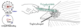
The reason for this is the different electric charges – oppositely charged particles attract each other (Coulomb’s law), which you know from physics lessons and the last lesson. In the same way, thin plastic bags or balloons stick to a wall, especially if you have charged them beforehand by rubbing.

☞ Accumulations of electric charge cause electric fields, and a force acts on individual charges in this field.

1.2 The tendency towards equalization

In nature, every system strives for equalization so that all elements have the lowest possible energy level.
If there are many electrons but only a few protons at one place, we speak of a negative excess of charge carriers. At this place, there is a negative electric potential relative to a place with neutral electric potential (‘earth’, ‘ground’), and the system will use every opportunity to bring about a balanced state, namely along the path of least resistance. We can control the equalization of this potential difference by preparing such a path for the electrons, e.g. via electric lines and cables, or by blocking their path with insulators. If we do not do this and the electric potential becomes too great, the charges also find their way in an uncontrolled manner, e.g. in a lightning strike between clouds and the Earth’s surface.
Electric fields play an important role in this, which we will come back to later.

☞ An excess of electrons on one side and a deficit of electrons on the other lead to the tendency towards equalization of charge carriers between the different electric potentials.

This is how voltage arises.

1.3 Voltage

In electrical engineering systems, voltage is the driving force that moves the electrons through the electric conductor – analogous to a loudspeaker announcement that makes people move from one place to another (example: a short-notice platform change of a train at the station).

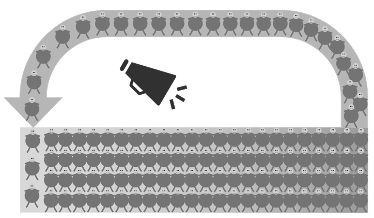
In the water analogy, voltage is the pressure with which the water is pushed through a pipe.

Physically, voltage is the energy per charge that is expended to move charge carriers from one point to another:

$$U=\frac{W}{Q}$$

One volt therefore means that one joule of energy is transferred per coulomb of electric charge ($1\mathrm{V}=1J/C$).

The quantity symbol of electric voltage is $U$. It is given in the unit volt with the unit symbol $\mathrm{V}$.

1.4 Resistance

On their way to the other platform, people have to pass unavoidable bottlenecks at stairs, doors and bends. The other people also slow down the movement: the more people there are, the more slowly individuals make progress.

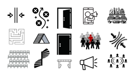
In electrical engineering, the electrons encounter bottlenecks on their way through the conductor, e.g. in the form of resistors installed specifically for this purpose, or at other components that form an unavoidable resistance, e.g. contact points such as plugs or switches.

In the water analogy, resistance is a narrow point created, for example, by the pipe itself, a valve or a kink.

The quantity symbol of electrical resistance is $R$.
Its unit is the ohm, abbreviated with the Greek capital letter $\Omega$ (‘omega’).

The reciprocal of resistance is called conductance. High resistance, low conductance; low resistance, high conductance. Its quantity symbol is the letter $G$. It has the unit siemens with the unit symbol $\mathrm{S}$.

1.5 Current

Depending on how high the voltage is and how large the resistances are, a certain number of electrons per unit of time is pushed through a certain point in the conductor. This is how current flow arises, and a certain current results. More specifically: the higher the voltage, the greater the current. The higher the resistance, the lower the current.

In the water analogy, current is the volume flow rate, i.e. the quantity of water molecules flowing at a certain point.

Mathematically, current is the electric charge per unit of time that flows through a conductor cross-section:

$$I=\frac{\Delta Q}{\Delta t}$$

One ampere means that one coulomb of electric charge flows through the conductor cross-section per second ($1\mathrm{A}=1C/s$).

Technical current direction

In electrical engineering, the technical current direction (German: technische Stromrichtung; also: conventional current direction) is used. It runs from the positive terminal to the negative terminal – i.e. opposite to the actual direction of movement of the electrons, which travel from the negative terminal to the positive terminal (cf. EE1-01).

This convention has historical reasons and is binding worldwide in electrical engineering. All current arrows in this script point in the technical current direction.

The quantity symbol of electric current is $I$.
Its unit is the ampere, abbreviated with the unit symbol A.

1.6 Ohm’s law

The relationship between voltage and current is proportional: the higher the voltage, the greater the current.

$$U\sim I$$

The proportionality factor is the resistance. Like almost everything in electrical engineering, this relationship between voltage, resistance and current can be expressed by a formula that you already know from physics lessons, Ohm’s law:

$$U=R\cdot I$$

(read: ‘$U$ equals $R$ times $I$.’ or ‘$U$ equals the product of $R$ and $I$.’ )
This formula (also known as the ‘URI’ formula) is used above all to calculate the voltage for a given resistance and current.

where:

• $U$ the voltage in volts ($\mathrm{V}$)
• $R$ the resistance in ohms ($\Omega$)
• $I$ the current in amperes ($\mathrm{A}$)

Details on the quantities

For every quantity that appears in this script, there is a separate page on which it is introduced in detail with its quantity symbol, unit, unit symbol and further relevant details. These detail pages are linked in each case. I recommend that you look at this page to clear up any questions that may arise when you read the texts and formulas here in the lesson.
🔗 All electrical quantities

By mathematical transformation (equivalence transformation), Ohm’s law can also be written in this form:

$$I=\frac{U}{R}$$

(read: ‘$I$ equals $U$ over $R$.’ or ‘$I$ equals the quotient of $U$ and $R$.’ )

Here the voltage is in the numerator. The greater the voltage, the greater the current. The resistance is in the denominator. The greater the resistance, the smaller the current. This formula is used above all to calculate the current for given values of voltage and resistance.

A further rearrangement leads to this formulation, which is used above all to calculate the resistance for given values of voltage and current:

$$R=\frac{U}{I}$$

(read: ‘$R$ equals $U$ over $I$.’ or ‘$R$ equals the quotient of $U$ and $I$.’ )

The conductance is the reciprocal of the resistance:

$$G=R^{-1}=\frac{1}{R}=\frac{I}{U}$$

(read: ‘$G$ equals $R$ to the power of -1 or equals 1 over $R$.’)

Theoretical context

In its general form, Ohm’s law reads:

$$\vec{E}=\sigma \cdot \vec{J}$$

where:

• $\vec{E}$ the electric field strength
• $\sigma$ the conductivity tensor of the medium through which the current flows
• $\vec{J}$ the current density

In isotropic (not dependent on direction) and linear (not dependent on influencing quantities) media, the electrical conductivity can be regarded as a scalar (one-dimensional quantity). The conduction of current is then proportional to the electric field that causes the current flow, and it lies in the same direction. In this case, the simple Ohm’s law applies.

1.7 Power and efficiency

We know the power rating of motor vehicles in kilowatts (kW) and, from earlier times, also in metric horsepower (PS). Many household appliances also carry a rating for the power that the appliance draws in operation, e.g. ‘1 000–1 200 W’ on a travel hair dryer.

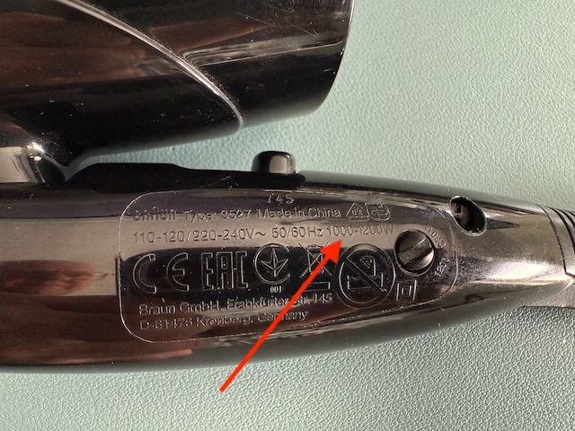
The quantity symbol of power is the letter $P$. In electrical engineering, it is generally defined as the product of current and voltage:

$$P=U\cdot I$$

The unit of electric power is the watt with the unit symbol $\mathrm{W}$.

In combination with Ohm’s law ($U=R\cdot I$ or $I=\frac{U}{R}$), power can also be formulated as follows:

$$P=I^2\cdot R$$ $$P=\frac{U^2}{R}$$

Here, too, the following applies: if two of the three quantities in an equation are given, you can calculate the third.

Back to the heating device.

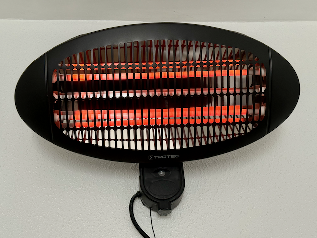
The heating device draws electric power (according to the rating plate, max. 2 000 W) and releases it mainly as heat (thermal power). – Why ‘mainly’? We not only feel the heat but also see that the heating rods glow. In other words: most of the power ($\gg 99\%$) is emitted in the form of warming infrared radiation that is invisible to the human eye, while a small part of the power ($\ll 1\%$) is emitted as radiation in the range of visible light.

The part of the power that does not go into the intended function is called power loss (German: Verlustleistung). And the ratio between input power and the power output in accordance with the function is called efficiency.

Expressed in formulas:

$$\eta =\frac{P_{out}}{P_{in}}$$ $$P_{out}=P_{in}\cdot \eta$$ $$P_{loss}=P_{in}\cdot (1-\eta )$$ $$P_{\mathrm{loss}}=P_{in}-P_{out}$$

where:

• $\eta$ the efficiency as a decimal number ($0<\eta <1$) or in %
• $P_{out}$ the power output in accordance with the function (at the heating rod the heat, at the lamp the light, at the electric motor the movement)
• $P_{in}$ the input power (the power that the device draws from the grid)
• $P_{loss}$ the power loss (at the heating rod the visible light, at the lamp and at the electric motor the heat)

In the case of the heating rod mentioned above, let us assume, for example, an efficiency of $\eta =0.995=99.5\%$; the power loss at level II is then:

$$P_{loss}=P_{in}\cdot (1-\eta )=1762\mathrm{W}\cdot (1-0.995)=1762\mathrm{W}\cdot 0.005=8.81\mathrm{W}\approx \underline{9\mathrm{W}}$$

Is 9 W a lot?

In percentage terms, $9\mathrm{W}$ is not much here and can practically be neglected in this context. In other contexts, however, $9\mathrm{W}$ cannot be neglected, because this power is enough to light up a dark driveway at night with an LED lamp or to charge a smaller tablet.

Speaking of ‘LED’ (light emitting diode) or ‘charging a tablet’ – power loss is usually released in the form of heat, for example:

• The smartphone’s rechargeable battery and the charger become warm or even hot during charging.
• An incandescent bulb becomes extremely hot in operation; an LED lamp also becomes warm to hot. (Here it is exactly the other way round from the heating device, where the glow makes up the losses.)
• The electric motor of an electric vehicle heats up moderately to strongly in operation, as does the rechargeable battery – not only during charging but also during discharging.

We will discuss the cause of the heat generation in the rechargeable battery in the lesson EE1-03 Sources.

Let us now take a look at the energy cost of operating the heating device from the example.

1.8 Energy and cost

Energy is traded on the market. In electrical engineering, energy is also referred to as work. The so-called energy meter (colloquially ‘electricity meter’) records the energy drawn in the household, and the so-called energy price is the basis for billing by the energy supplier.

Energy is the power drawn by a system over a period of time. As a formula:

$$W=P\cdot t$$

where:

• $W$ the energy in kilowatt hours ($\mathrm{kWh}$) or joules ($\mathrm{J}$)
• $P$ the power in watts ($\mathrm{W}$)
• $t$ the time in seconds ($\mathrm{s}$)

If you leave the heating device described above switched on at level 2 for one hour, this results in an energy ‘consumption’ of:

$$W=P\cdot t=1762\mathrm{W}\cdot 1\mathrm{h}=1762\mathrm{Wh}=\underline{1.762\mathrm{kWh}}$$

At an energy price of $0.29EUR/kWh$, the cost $K$ of one hour of heating is:

$$K=W\cdot p=1.762\mathrm{kWh}\cdot 0.29EUR/kWh=1.762\cdot 0.29\frac{\mathrm{kWh}\cdot \mathrm{EUR}}{\mathrm{kWh}}\approx \underline{0.51\mathrm{EUR}}$$

where:

• $W$ the energy or electrical work in kilowatt hours ($\mathrm{kWh}$)
• $K$ the cost in euros ($\mathrm{EUR}$)
• $p$ the energy price in euros ($\mathrm{EUR}$)

---

You now know ten fundamental electrical quantities and what they stand for:

• Electric charge
• Electric field strength
• Voltage
• Resistance
• Conductance
• Current
• Power
• Energy
• Efficiency
• Cost

In the following lessons, these partly simplified ideas will be deepened, and the physical phenomena and their mathematical representation will be made more precise and supplemented.

These ten quantities can now serve as examples to present the general rules that apply to professional (above all written) communication in electrical engineering.

2 Forms of representation of electrical engineering phenomena

Electrical engineering phenomena can be described in seven different ways:

• Verbal description
• Photo
• Simulation model
• Sketch/equivalent circuit diagram
• Graph/diagram
• Equation/formula
• Table

An electric heating device serves as an example. In the following, you can easily see that each form of representation contains certain information about the system. Not all information is contained in every form of representation.

2.1 Verbal description

‘An electric heater with two separately switchable heating rods is connected to a standard household socket-outlet via a supply cable approx. $1\mathrm{m}$ long with a protective-contact plug. When both heating rods are switched on (level 2), a current of approx. $7.66\mathrm{A}$ (measured) flows through the supply cable. At level 1, only one heating rod is switched on; a current of $3.83\mathrm{A}$ can then be measured in the supply cable.’

2.2 Photo

The photo shows a heating device with two red-glowing heating rods. At the bottom edge, you can see the supply cable and the cord switch, which is set to level 2.

2.3 Simulation model

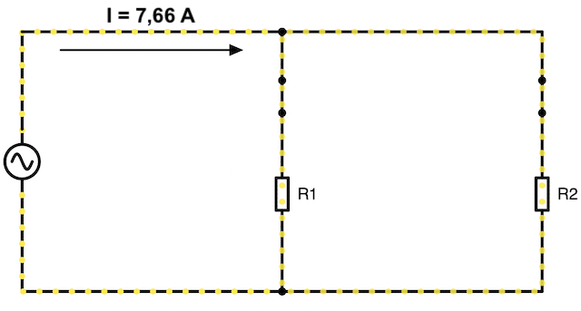
The simulation model shows the parallel connection of two resistors $R_1$ and $R_2$, each of which is in series with a closed switch ($S_1$ and $S_2$). The electric circuit is supplied by an AC voltage source. A total current $I=7.66\mathrm{A}$ flows.

2.4 Sketch

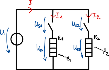
The sketch shows an equivalent circuit diagram of the heating device with:

• the power grid as a voltage source with the voltage $U$,
• the two heating rods as ohmic resistors (here: heating resistors $R_1$ and $R_2$) in parallel connection, across which the voltages $U_{R1}$ and $U_{R2}$ drop
• the switches ($S_1$, $S_2$), each in series with one of the heating rods, across which the voltages $U_{S1}$ and $U_{S2}$ drop,
• the currents $I$ (total current) as well as $I_1$ and $I_2$, which flow in the branches of the parallel connection,
• the powers $P_1$ and $P_2$, which are taken up by the heating resistors and given off as heat.

By convention, the components and connections are sketched in black, the voltages as voltage arrows in blue and the currents as current arrows in red.
(The representation of the individual components will be discussed in detail later on.)

Reference-arrow systems

Current and voltage arrows in schematics do not show the physical direction of motion of the charge carriers; instead, they define a reference direction (German: Bezugsrichtung, also: Zählrichtung). Whether the actual value turns out positive or negative follows from the calculation.

For components, there are two conventions for assigning the current arrow and the voltage arrow:

Load reference-arrow system (German: Verbraucherzählpfeilsystem):
The current arrow and the voltage arrow point in the same direction. This convention is used for loads (German: Verbraucher) (resistors, capacitors, inductors). In the load reference-arrow system, an ohmic resistor gives: $U=R\cdot I$ (positive sign).

Generator reference-arrow system (German: Erzeugerzählpfeilsystem):
The current arrow and the voltage arrow point in opposite directions. This convention is used for sources (German: Quellen) (voltage sources and current sources).

Mnemonic

• Load reference-arrow system: current flows into the positive terminal → the component takes up power ($P=U\cdot I>0$).
• Generator reference-arrow system: current flows out of the positive terminal → the source delivers power ($P=U\cdot I>0$).

In this script – unless stated otherwise – the load reference-arrow system is used.

2.5 Graph

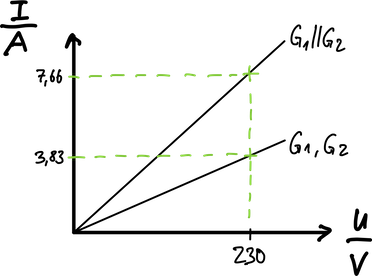
The graph shows the current-voltage characteristic curves of the heating device. Each heating rod is an ohmic resistor.

• The lower straight line belongs to a single heating rod with the resistance $R$. The slope of the characteristic curve corresponds to the conductance $G=\frac{1}{R}$.
• The upper straight line represents both heating rods in parallel connection.

In general: the greater the conductance (i.e. the smaller the resistance), the steeper the $I(U)$ characteristic curve.

2.6 Equation

In equations, the physical quantities are not written out but are represented by so-called quantity symbols. You can find the quantity symbols, units, etc. on the detail pages for the respective quantities. In the following calculation examples, I use the quantity symbols ‘just like that’ and rely on the procedure being familiar to you from maths and physics lessons.

Given:
Mains voltage $U=230\mathrm{V}$
Measured current $I=7.66\mathrm{A}$

Calculations:
Resistance of both heating rods in parallel connection:

$$R_{tot}=\frac{U}{I}=\frac{230\mathrm{V}}{7.66\mathrm{A}}\approx \underline{30.0\Omega }$$

The conductance (see also graph):

$$G_{\text{tot}}=\frac{1}{R_{tot}}=\frac{1}{30.0\Omega }\approx \underline{33.3\mathrm{mS}}$$

Power at level I (one heating rod):

$$P_1=U\cdot I_1=230\mathrm{V}\cdot \frac{7.66\mathrm{A}}{2}\approx \underline{881\mathrm{W}}$$

Power at level II (two heating rods):

$$P=P_{12}=U\cdot I=U\cdot 2\cdot I_1=230\mathrm{V}\cdot 7.66\mathrm{A}\approx \underline{1762\mathrm{W}}$$

Cost

2.7 Table

The table summarizes the verbally described measurement results (currents) together with calculated values (powers):

	Rod 1 ON	Rod 2 ON	Both rods ON
Voltage	$230\mathrm{V}$	$230\mathrm{V}$	$230\mathrm{V}$
Supply cable current	$3.83\mathrm{A}$	$3.83\mathrm{A}$	$7.66\mathrm{A}$
Resistance	$60\Omega$	$60\Omega$	$30\Omega$
Conductance	$16.7\mathrm{mS}$	$16.7\mathrm{mS}$	$33.3\mathrm{mS}$
Power	$881\mathrm{W}$	$881\mathrm{W}$	$1762\mathrm{W}$

☞ You can take different information about the phenomenon or the system from the different forms of representation. In this script, the tasks mostly use a combination of verbal description (possibly with a photo), sketch and equations. Graphs or tables occasionally supplement the task or its solution.

3 Notation of electrical quantities

This script uses 37 quantities from electrical engineering alongside some physical and material-dependent quantities and constants. In this and the previous lesson, the following ten quantities were introduced:

• Electric charge (EE1-01)
• Electric field strength (EE1-01)
• Voltage
• Resistance
• Conductance
• Current
• Power
• Energy
• Efficiency
• Cost

Each quantity has its own page on which it is introduced in detail with its quantity symbol, unit and other relevant details. These detail pages are linked in each case. I recommend that you look at these pages to clarify any questions that may arise when you read the texts and formulas in the lessons.

In the calculation examples above, numerous rules on the notation of electrical quantities can be recognized implicitly. So that you can do everything correctly in future, I explain these rules in detail and explicitly below.

3.1 Values

As with all physical quantities, electrical values are given as the product of a numerical value and a unit or dimension.

Mathematically, a quantity $G$ is written as the product of the numerical value $\{G\}$ and the dimension $[G]$:

$$G=\{G\}\cdot [G]$$

e.g. for the voltage:

$$U=\{U\}\cdot [U]=230\cdot \mathrm{V}=230\mathrm{V}$$

with $\{U\}=230$ and $[U]=V$.

The curly brackets stand for the mathematical function ‘value of’.
The square brackets stand for the mathematical function ‘dimension of’ or ‘unit of’.

NOTE

Although you often see in technical subjects that the unit itself is written in square brackets, e.g. as an axis label on a diagram, strictly speaking this is not mathematically correct.

The unit is abbreviated by a unit symbol, e.g. $230\mathrm{V}$ for the voltage present at a standard household socket-outlet. Here, $230$ is the numerical value and $\mathrm{V}$ is the unit symbol for the unit volt. The multiplication sign between the numerical value and the unit symbol is omitted – this is common practice in engineering. On a computer, a no-break space is used instead of the multiplication sign so that no line break can occur between the value and the unit symbol.

3.2 Quantity symbols

When you calculate with quantities, quantity symbols (German: Formelzeichen) are used in equations instead of the written-out quantity, e.g. $U$ for the voltage in the equation of Ohm’s law $U=R\cdot I$.

Unlike unit symbols, quantity symbols are set in italics.

Since considerably more quantity symbols are needed for technical quantities than the German alphabet has letters, electrical engineering also makes use of the letters of the Greek alphabet, such as $\omega$ (‘omega’) for angular frequency.

Greek alphabet

Because in engineering we need more than 26 letters to write quantity symbols and unit symbols, Greek letters are also used.

Name	Uppercase	Lowercase	Lowercase (alternative)
Alpha	$A$	$\alpha$
Beta	$B$	$\beta$
Gamma	$\Gamma$	$\gamma$
Delta	$\Delta$	$\delta$
Epsilon	$E$	$ϵ$	$\epsilon$
Zeta	$Z$	$\zeta$
Eta	$H$	$\eta$
Theta	$\Theta$	$\theta$	$\vartheta$
Iota	$I$	$\iota$
Kappa	$K$	$\kappa$	$\varkappa$
Lambda	$\Lambda$	$\lambda$
Mu	$M$	$\mu$
Nu	$N$	$\nu$
Xi	$\Xi$	$\xi$
Omicron	$O$	$o$
Pi	$\Pi$	$\pi$	$\varpi$
Rho	$P$	$\rho$	$\varrho$
Sigma	$\Sigma$	$\sigma$	$\varsigma$
Tau	$T$	$\tau$
Upsilon	${\rm Y}$	$\upsilon$
Phi	$\Phi$	$\varphi$	$\phi$
Chi	$X$	$\chi$
Psi	$\Psi$	$\psi$
Omega	$\Omega$	$\omega$

Uppercase and lowercase letters

If the quantity is constant, i.e. it does not change over time, electrical engineering uses the uppercase letter as the quantity symbol, e.g. $I$ for the current of a direct current and also for the RMS value of an alternating current.

For time-dependent quantities, lowercase letters are used,
e.g. $i(t)=\hat{i}\cdot \sin (\omega t)$ for the time-varying, sinusoidal current with the peak value $\hat{i}$ and the angular frequency $\omega$.

Complex quantities with a phase difference (‘phasors’) are represented by underlined quantity symbols, e.g. $\underline{U}=20\mathrm{V}+j5\mathrm{V}$ for the complex voltage in an AC circuit.

3.3 Precision

The precision with which values are given depends on the precision of the source data. For measurements, the precision depends on the resolution of the measuring instruments. For calculations, it depends on how precisely the values are given and in which order of magnitude they lie.

It is not primarily about decimal places, but about significant digits (German: signifikante Stellen). Significant digits are the digits of a number that provide meaningful information about its precision.

$U=12.3\mathrm{V}$ has three significant digits, but only one decimal place.
$R=42\Omega$ has two significant digits with zero decimal places.

Calculations should be carried out in such a way that the final result does not have more significant digits than the least precise value in the task allows. In addition, the general rules of rounding apply.

Caution!

Calculators display decimal places that go beyond the precision of the values entered and therefore must not be regarded as significant. In other words: calculators ‘invent’ decimal places.
Feel free to continue calculating with all decimal places in memory, but at the end, it makes sense to give the result only with the significant digits.

In the exercises for this script, the values are generally given exactly with their significant digits.

Example

Given are the voltage $U=11.8\mathrm{V}$ across a component and its resistance $R=470\Omega$.
Required is the current $I$ that flows through the component.

Calculation:
From Ohm’s law it follows that:

$$I=\frac{U}{R}=\frac{11.8\mathrm{V}}{470\Omega }=0.0251\mathrm{A}\approx \underline{25.1\mathrm{mA}}$$

The correct result (underlined) has three significant digits, just like the given values. To achieve this precision when using the unit ampere ($\mathrm{A}$) – without the prefix ‘milli’ ($\mathrm{m}$) – four decimal places must be given. By using the SI prefix ‘milli’ ($10^{-3}$), the value can be given in the unit $\mathrm{mA}$ with one decimal place, which is practical and easy to read.

The example shows that it is not the number of decimal places that matters; rather, the precision depends on the number of significant digits.

You should continue calculating with at least this precision. It makes sense to continue calculating with the value stored in the calculator (here: $0.02510638298$). However, the solution should not be given more precisely than the source data allow.

3.4 Units

In all calculations in this script, you always calculate with units. I often find that this aspect of calculation, which is important from an engineering point of view, gets too little attention in mathematics lessons. Yet calculating with units is such an important instrument for assessing the correctness of your own calculations – and, incidentally, of calculations by AI models too!!! Very many conceptual and computational errors in working on tasks become apparent when you set up the unit equation.

NOTE:

To avoid errors, always calculate with units!

Example

The calculation from EE1-01 on the Coulomb force provides a good example of the benefit of calculating with units:

$$F=8.988\cdot 10^9\frac{\mathrm{N}\cdot {\mathrm{m}}^2}{{\mathrm{C}}^2}\cdot \frac{1\cdot 10^{-18}}{25\cdot 10^{-8}}\frac{{\mathrm{C}}^2}{{\mathrm{m}}^2}=35.96\cdot 10^{-3}\frac{\mathrm{N}\cdot {\mathrm{m}}^2\cdot {\mathrm{C}}^2}{{\mathrm{m}}^2\cdot {\mathrm{C}}^2}=35.96\cdot 10^{-3}\mathrm{N}\approx \underline{36\mathrm{mN}}$$

Because all quantities appear in the calculation with their units, you can see very clearly how, by cancelling the units above and below the fraction line, newton remains at the end as the unit of force. In this way, you can be sure that you have inserted the correct constant and taken all factors into account.

NOTE

In the exam, I award points for giving values with the correct unit. If the correct unit is missing, points are lost. I therefore recommend that you get used to writing down the units and calculating with units right from the start.

The result $F=36\mathrm{mN}$ contains the unit prefix ‘milli’. Unit prefixes are standardized as SI prefixes in the SI system, as I show in the next section.

3.5 SI prefixes

In engineering, powers of ten are also referred to as orders of magnitude. Many calculators allow you to enter values with these powers of ten. Each order of magnitude is assigned a prefix symbol (SI prefix), which is placed in front of the unit.

SI prefix	Name	Power	Number word	Number
Y	yotta	$10^{24}$	septillion	1 000 000 000 000 000 000 000 000
Z	zetta	$10^{21}$	sextillion	1 000 000 000 000 000 000 000
E	exa	$10^{18}$	quintillion	1 000 000 000 000 000 000
P	peta	$10^{15}$	quadrillion	1 000 000 000 000 000
T	tera	$10^{12}$	trillion	1 000 000 000 000
G	giga	$10^9$	billion	1 000 000 000
M	mega	$10^6$	million	1 000 000
k	kilo	$10^3$	thousand	1 000
–	–	$10^0$	one	1
m	milli	$10^{-3}$	thousandth	0.001
µ	micro	$10^{-6}$	millionth	0.000 001
n	nano	$10^{-9}$	billionth	0.000 000 001
p	pico	$10^{-12}$	trillionth	0.000 000 000 001
f	femto	$10^{-15}$	quadrillionth	0.000 000 000 000 001
a	atto	$10^{-18}$	quintillionth	0.000 000 000 000 000 001
z	zepto	$10^{-21}$	sextillionth	0.000 000 000 000 000 000 001
y	yocto	$10^{-24}$	septillionth	0.000 000 000 000 000 000 000 001

SI prefixes are written without a space before the unit symbol and, like the unit symbol, in upright, non-italic type, e.g. $63\mathrm{k}\Omega =63\cdot 10^3\Omega =63000\Omega$.

To avoid confusion between the unit metre (m) and the prefix for milli (m), the metre is always placed at the end of the units, while the prefix for milli (10-3) comes at the front (a PREfix, after all). Accordingly, $\mathrm{mV}$ stands for millivolt and $\mathrm{Vm}$ for volt metre (strictly speaking $\mathrm{V}\cdot \mathrm{m}$).

In German, the micrometre ($\mu \mathrm{m}$) is also called by the name of the Greek letter for short (German: Mü [myː]); in English, the Greek letter $\mu$ is pronounced [mju:]. In addition, micron (mc) is also common in English for the micrometre.

The detail pages on the quantities always also contain the typical orders of magnitude and examples of the corresponding SI prefixes.

NOTE

In exams, I mark quantities given with a unit in the wrong order of magnitude (with the wrong SI prefix) as wrong and deduct points for them.

4 Scalars, vectors and tensors

In electrical engineering, we encounter three categories of mathematical quantities that differ in their complexity: scalars, vectors and tensors. These form a hierarchy in which each category is a special case of the next higher one.

4.1 Scalars (zeroth-order tensors)

A scalar (German: Skalar) is a quantity that is fully described by a single number with a unit. Scalars have no direction – they are the same in all coordinate systems.

Examples from electrical engineering:

• Voltage: $U=230\mathrm{V}$
• Resistance: $R=47\mathrm{k\Omega }$
• Power: $P=100\mathrm{W}$
• Temperature: $T=25°C$
• Energy: $W=3.6\mathrm{kJ}$

4.2 Vectors (first-order tensors)

A vector (German: Vektor) is a quantity with magnitude and direction. In 3D, we need three components for a complete description. When the coordinate system is changed, vectors transform according to certain rules.

Representation:

$$\vec{E}=\left(\begin{array}{c}{E}_x\\ E_y\\ E_z\end{array}\right)=E_x\cdot {\vec{e}}_x+E_y\cdot {\vec{e}}_y+E_z\cdot {\vec{e}}_z$$

Here, ${\vec{e}}_{x,y,z}$ are the unit vectors in the x, y and z directions.

Examples from electrical engineering:

• Electric field strength: $\vec{E}$ in $V/m$
• Current density: $\vec{J}$ in $A/{\mathrm{m}}^2$
• Force: $\vec{F}$ in $\mathrm{N}$

Intuitively:

• A vector is like an arrow in space – it points in a certain direction and has a certain length.
• If someone pushes you, your movement has a certain direction and a certain intensity (force).

4.3 Tensors (second and higher order)

A second-order tensor (German: Tensor 2. Stufe) links two vectors with each other. In 3D, it is represented by a 3×3 matrix with 9 components. Tensors describe direction-dependent properties of materials.

Representation as a matrix:

$$\overleftrightarrow{\epsilon }=\left(\begin{array}{ccc}{\epsilon }_{xx}& {\epsilon }_{xy}& {\epsilon }_{xz}\\ {\epsilon }_{yx}& {\epsilon }_{yy}& {\epsilon }_{yz}\\ {\epsilon }_{zx}& {\epsilon }_{zy}& {\epsilon }_{zz}\end{array}\right)$$

Examples from electrical engineering:

• Permittivity tensor $\overleftrightarrow{\epsilon }$ in anisotropic crystals: $\vec{D}=\overleftrightarrow{\epsilon }\cdot \vec{E}$
• Conductivity tensor $\overleftrightarrow{\sigma }$ in semiconductors: $\vec{J}=\overleftrightarrow{\sigma }\cdot \vec{E}$
• Piezoelectric tensor $\overleftrightarrow{d}$ in piezoelectric crystals: $\vec{D}=\overleftrightarrow{d}\cdot \overleftrightarrow{T}$

where:

• $\vec{D}$ is the electric flux density in $C/{\mathrm{m}}^2$
• $\vec{E}$ is the electric field strength in $V/m$
• $\vec{J}$ is the current density in $A/{\mathrm{m}}^2$
• $\overleftrightarrow{T}$ is the mechanical stress tensor in $N/{\mathrm{m}}^2$ (describes tensile, compressive and shear forces in the material)
• $\overleftrightarrow{\epsilon }$ is the permittivity tensor in $F/m$ (dielectric property)
• $\overleftrightarrow{\sigma }$ is the conductivity tensor in $S/m$ (electric conductivity)
• $\overleftrightarrow{d}$ is the piezoelectric tensor in $C/N$ or $m/V$ (coupling between mechanical stress and electric flux density)

Intuitively:

• A tensor describes how a property behaves differently depending on the direction – like a wooden board that has different properties along the grain than across it.
• If you swim in a river, you experience different flow forces depending on where you are swimming:
  • the position along the course of the river (x),
  • the distance from the bank (y) and
  • the water depth (z) determine the flow forces.

4.4 The hierarchy at a glance

Order	Name	Components (3D)	Example	Application
0	Scalar	1	$R=100\mathrm{\Omega }$	Isotropic materials
1	Vector	3	$\vec{E}=(0,0,5)V/m$	Fields in space
2	Tensor	9	$\overleftrightarrow{\epsilon }$	Anisotropic materials

4.5 Practical significance in electrical engineering

In the fundamentals (isotropic materials, homogeneous fields):

$$D=\epsilon \cdot E$$

The permittivity $\epsilon$ is a scalar – the material behaves the same in all directions.

In advanced applications (anisotropic crystals, inhomogeneous fields):

$$\vec{D}=\overleftrightarrow{\epsilon }\cdot \vec{E}$$

The permittivity $\overleftrightarrow{\epsilon }$ is a tensor – the electric field in the x direction can cause a displacement in the y direction!

4.6 Mnemonic

Scalar: ‘How much?’ – A number
Vector: ‘How much and where to?’ – An arrow in space
Tensor: ‘How much where to, when excited from where?’ – A direction-dependent link

In the fundamentals of electrical engineering, we mainly work with scalars and simplified vectors. Tensors only become relevant for special materials (crystals, ferrites, prestressed materials) or when we model the general case (not a simplified special case).

5 Vector and scalar quantities in electrical engineering

In nature, many quantities in electrical engineering are vector quantities with a magnitude and a direction, and some are even tensors, as shown above. In the introductory lectures on electrical engineering, however, we mostly calculate with scalar quantities. Here I explain why and when this simplification is permissible.

5.1 The physical reality

In nature, electric and magnetic fields are always vectorial. An electron in an electric field ‘feels’ not only how strongly it is pulled, but also in which direction. A complete description therefore requires vector quantities:

• Electric field strength: $\vec{E}(\vec{r})$
• Electric flux density: $\vec{D}(\vec{r})$
• Magnetic field strength: $\vec{H}(\vec{r})$
• Magnetic flux density: $\vec{B}(\vec{r})$
• Current density: $\vec{J}(\vec{r})$
• Force: $\vec{F}$

5.2 Overview of the vector quantities in the fundamentals of electrical engineering

Primarily vector quantities

These quantities are vectors by nature, but are often treated as scalars in the fundamentals:

Quantity	Vector form	Scalar form	Typical application
Electric field strength	$\vec{E}$	$E$	Parallel-plate capacitor
Electric flux density	$\vec{D}$	$D$	Dielectric
Magnetic field strength	$\vec{H}$	$H$	Long inductor
Magnetic flux density	$\vec{B}$	$B$	Air gap
Current density	$\vec{J}$	$J$	Straight conductor
Force	$\vec{F}$	$F$	Coulomb force

Scalars from vector operations

These quantities are scalars that result from the integration of vector fields:

• Voltage: $U=\int \vec{E}\cdot d\vec{s}$ (line integral of the field strength)
• Electric flux: $\Psi =\int \vec{D}\cdot d\vec{A}$ (surface integral of the electric flux density)
• Magnetic flux: $\Phi =\int \vec{B}\cdot d\vec{A}$ (surface integral of the magnetic flux density)
• Current: $I=\int \vec{J}\cdot d\vec{A}$ (surface integral of the current density)

5.3 Conditions for the scalar simplification

The simplification from vector quantities to scalar quantities is not cheating, but a justified reduction for special geometries. It is permissible if at least one of the following conditions is met:

One-dimensional geometry

The field direction is determined by the arrangement:

• Parallel-plate capacitor: the field always points from the positive to the negative plate
• Coaxial cable: the field points radially outwards
• Long inductor: the magnetic field is parallel to the inductor axis

Parallelism ensured

All relevant vectors point in the same direction:

• $\vec{E}$ and $\vec{D}$ are parallel (in homogeneous media)
• Field lines and surface normal are parallel
• The scalar product then becomes a simple product: $\vec{D}\cdot \vec{A}=D\cdot A$

Only magnitudes relevant

The information about the direction is not needed for the calculation:

• Energy calculations: $W=\frac{1}{2}C{U}^2$
• Capacitance determinations: $C=\epsilon \cdot A_C/d$
• Resistance calculations: $R=\rho \cdot l/A_{\mathrm{cond}}$

where:

• $W$ the stored electric energy in $\mathrm{J}$ (joules)
• $C$ the capacitance of the capacitor in $\mathrm{F}$ (farads)
• $U$ the voltage across the capacitor in $\mathrm{V}$ (volts)
• $\epsilon$ the permittivity of the dielectric in $F/m$ (farads per metre), with $\epsilon ={\epsilon }_0\cdot {\epsilon }_r$
  • ${\epsilon }_0$ the permittivity of vacuum (electric field constant) ${\epsilon }_0\approx 8.8542\cdot 10^{-12}\text{F/m}$
  • ${\epsilon }_r$ the relative permittivity (permittivity of the material relative to vacuum) ${\epsilon }_r$
    • vacuum/air: ${\epsilon }_r\approx 1$
    • simple dielectrics: ${\epsilon }_r\approx 3\text{–}7$
• $A_C$ the plate area of the capacitor in ${\mathrm{m}}^2$ (square metres)
• $d$ the plate separation of the capacitor in $\mathrm{m}$ (metres)
• $R$: resistance in $\mathrm{\Omega }$ (ohms)
• $\rho$: resistivity of the material in $\mathrm{\Omega }\cdot \mathrm{m}$ (ohm metres)
• $l$: length of the conductor in $\mathrm{m}$ (metres)
• $A_{\mathrm{cond}}$: cross-sectional area of the conductor in ${\mathrm{m}}^2$ (square metres)

We then speak of homogeneous fields (see EE1-01).

5.4 The simplification hierarchy

Fully vectorial: $\vec{D}(\vec{r})=\epsilon \cdot \vec{E}(\vec{r})$
↓ (homogeneous field)
Direction known: $D=\epsilon \cdot E$ (with sign)
↓ (only magnitudes relevant)
Purely scalar: $D=\epsilon \cdot E$ (positive values only)

5.5 Concrete examples

Example: parallel-plate capacitor (simplification permitted)

Complete vectorial description:

$$\vec{E}=-\frac{U}{d}\cdot {\vec{e}}_x$$ $$\vec{D}=\epsilon \cdot \vec{E}=-\epsilon \cdot \frac{U}{d}\cdot {\vec{e}}_x$$

Simplified scalar calculation:

$$E=\frac{U}{d}$$ $$D=\epsilon \cdot E=\epsilon \cdot \frac{U}{d}$$

The simplification is permissible because:

• the field between the plates is homogeneous.
• the direction is determined by the geometry.
• we only calculate with magnitudes.

Counterexample (vector calculation required)

When superimposing two point charges, we have to calculate with vectors:

$${\vec{E}}_{tot}={\vec{E}}_1+{\vec{E}}_2=\frac{Q_1}{4\pi \epsilon r_1^2}\cdot {\vec{e}}_{r1}+\frac{Q_2}{4\pi \epsilon r_2^2}\cdot {\vec{e}}_{r2}$$

No simplification is possible here, because two different electric fields are superimposed and their field directions are therefore different.

5.6 Special cases – tensor quantities

In anisotropic materials, material properties can even become tensors (German: Tensoren):

• Permittivity $\epsilon$ → $\overleftrightarrow{\epsilon }$ (in crystals)
• Permeability $\mu$ → $\overleftrightarrow{\mu }$ (in ferrites)
• Conductivity $\sigma$ → $\overleftrightarrow{\sigma }$ (in semiconductors)

In the fundamentals, however, we treat these as scalar material constants.

5.7 The didactic message

We do not simplify here because the physics is simple, but because we choose clever geometries in which the vector property plays no role. This is engineering elegance that makes learning the fundamentals easier.

The scalar treatment in the fundamentals is a deliberate didactic decision:

1. It allows you to focus on the physical relationships.
2. It reduces the mathematical complexity.
3. It covers the most common practical applications.

5.8 Limits of the simplified approach

Later in your studies, full vector calculus becomes indispensable for:

• Maxwell’s equations in differential form,
• the calculation of electromagnetic waves,
• antenna radiation,
• numerical field calculations (FEM simulations),
• multiphase systems (three-phase systems).

The scalar relationships you learn in the fundamentals remain valid as special cases and form the foundation for a deeper understanding of vectorial field theory.

---

Exercises for this chapter

Exercise EE1-02.01 – Electric charge, voltage and energy of a rechargeable battery
Exercise EE1-02.02 – Electric potentials and voltage
Exercise EE1-02.03 – Plant lighting, power and efficiency
Exercise EE1-02.04 – Case fan schematic, symbols, calculation
Exercise EE1-02.05 – Current of a refrigerator

---

Classes from previous semesters

---

⏭️ Continue with: EE1-03 Sources 🔗