Representation and minimization of logic functions

Prof. Dr. Thorsten Jungmann (last updated 2026-10-20)

Overview of this lesson

---

What is this lesson about? – The guiding questions:

• How can a hand-drawn grid of zeros and ones make a logic circuit smaller and cheaper?
• Two circuits look completely different: how can you prove that they do exactly the same job?
• On a cold, sunny day, when should the energy from the photovoltaic (PV) system go into the hot-water tank and when into the lithium iron phosphate (LFP) battery – and how do you turn that rule into a circuit that can be produced efficiently?

---

What will you be able to do at the end of this lesson? – The intended learning outcomes:

• You synthesize circuits from a description of their function.
• You minimize circuits.
• You assess whether a circuit fulfils the required function.

---

What will you know at the end of this lesson? – The building blocks of knowledge:

• Representation of logic functions (normal forms)
• Algebraic minimization
• Minimization with the Karnaugh map

---

How is the content organized? – The structure:

• 1 From the description to the circuit – Combinational logic design
• 2 One term per row – Normal forms
• 3 Fewer gates, same function – Algebraic minimization
• 4 Zeros and ones in a grid – The Karnaugh map
• 5 Same job, different circuit? – Drawing and checking the circuit
• 6 Sun for the hot water or for the battery? – A complete design
• 7 What have you learnt? – Summary and answers to the guiding questions

Review of the previous lesson

In the previous lesson, you got to know the logic gates and learnt to calculate with 0 and 1.

• The basic gates NOT, AND and OR and the derived logic operations NAND, NOR, XOR and XNOR combine bits; each gate consists of a few transistors.
• Seven forms of representation describe the same function, among them the truth table, the logic expression and the Karnaugh map.
• The axioms and theorems of Boolean algebra, among them uniting and De Morgan’s laws, transform expressions.
• You analysed given circuits: from the circuit to its expression, its truth table and its timing behaviour.

Today, we go the other way: from a description of what a circuit is to do to the circuit itself – and we make the circuit as small as possible.

1 From the description to the circuit – Combinational logic design

1.1 From analysis to synthesis

In the previous lesson, you analysed circuits that someone else had designed: from the circuit to its expression, its truth table and its timing behaviour (DET-02, chapter 6). In practice, the task often runs the other way round [12, p. 23]. Someone describes in words what a circuit is to do, and you have to build it. Designing a circuit from a description of its function is called synthesis (German: Synthese) [5, pp. 93, 115]. LaMeres calls the whole process of creating a logic circuit from a word description or a truth table combinational logic design (German: Schaltungsentwurf): first, a circuit is derived directly from the truth table, then it is transformed into an equivalent circuit with fewer gates [5, p. 93]. Beuth and Beuth divide synthesis into five steps, from the description of the function to the minimized circuit [15, pp. 69–70]. In this module, the description is our starting point, and we use six steps (figure):

1. Define the inputs and the outputs as logic variables and state what a 1 means for each of them.
2. Set up the truth table: decide the output for every combination of the inputs.
3. Read a normal form (German: Normalform) from the table, an expression that describes the function completely.
4. Minimize the expression, so that the circuit needs as few gates as possible.
5. Draw the circuit, or describe it in VHDL.
6. Check that the circuit does what the description demands.

Compared with Beuth and Beuth, we write the normal form as a step of its own, minimize before we draw the circuit and add the check against the description [15, pp. 69–70]. Steps 1 and 2 need understanding: you turn sentences into ones and zeros, and the quality of the whole design depends on them [15, p. 69]. Steps 3 to 5 follow fixed rules; this is why tools can take them over [5, p. 155] (section 6.3). Step 6 completes the design: a circuit is only finished when you have shown that it meets the description, and if you find a deviation, you go back. LaMeres shows the classical design flow for a combinational circuit with similar stages, from the description through the truth table, the Karnaugh map and the minimized expression to the circuit [5, p. 163]. In his flow, the choice of a logic family and the placement and wiring of the gates come before the check; after it, the circuit is built [5, p. 163]. He calls the check verification [5, p. 161].

These six steps are the thread of this lesson, and chapters 2 to 6 each begin by naming the step that they cover. Chapter 1 covers steps 1 and 2, chapter 2 the normal forms of step 3, chapters 3 and 4 how to minimize in step 4, first with Boolean algebra and then with the Karnaugh map, and chapter 5 steps 5 and 6: the circuit and its check. Chapter 6 goes through all six steps once more with a complete design. Two examples run through the lesson: the ringtone of your smartphone in chapters 1 to 5, and in chapter 6 a rule that decides where the surplus energy of a photovoltaic system goes.

1.2 Steps 1 and 2: from the description to the truth table

Steps 1 and 2 turn the description into a truth table. Our example comes from DET-02, 3.1. There, your smartphone rang audibly only if it was not switched to silent – leaving aside the other settings of the phone. Now we take two of them into account. Silent mode mutes the ringtone for every call; at most, the phone vibrates. Do Not Disturb silences incoming calls as well, but it can make an exception for callers that you have marked as favourites. Silent mode has priority: when it is on, the phone stays silent even when a favourite calls.

Step 1 defines the variables. Each of them states what its 1 means:

• $A$: silent mode is on
• $B$: the caller is one of your favourites
• $C$: Do Not Disturb is on
• $Y$: the ringtone is audible

Step 2 decides the output for each of the $2^3=8$ combinations of the inputs, row by row, in the order that you know from DET-02, 2.2:

Row	$A$	$B$	$C$	$Y$
0	0	0	0	1
1	0	0	1	0
2	0	1	0	1
3	0	1	1	1
4	1	0	0	0
5	1	0	1	0
6	1	1	0	0
7	1	1	1	0

With silent mode on, the phone stays silent whatever the other inputs say: $Y=0$ in rows 4 to 7. With silent mode off, it rings unless Do Not Disturb blocks the call. It rings in row 0, where no setting is active, and in row 2, where a favourite calls. It stays silent in row 1, where Do Not Disturb is on and the caller is not a favourite. Row 3 is the exception: Do Not Disturb is on, but a favourite calls, so the phone rings.

Image by Qwen-Image 2.1

Think of a night with Do Not Disturb, as in the photo: the phone on the bedside table is to stay silent – unless one of your favourites calls. The example shows a typical difficulty of step 2. A description in words often leaves room for misunderstanding [15, p. 69]: does the exception for favourites also apply in silent mode? The truth table forces you to decide every single row, and a question that the description leaves open has to be clarified before you build anything [15, p. 69]. Here, the answer is row 7: silent mode wins.

2 One term per row – Normal forms

2.1 Minterms

Step 3 of synthesis (section 1.1) turns the truth table into an expression of a fixed, standard structure, a normal form [15, p. 72]. For this, we need two definitions. A literal (German: Literal) is a variable or its negation, such as $A$ or $\overline{A}$, in a logic expression [5, p. 115]. Each appearance counts as a literal of its own: the expression $\overline{A}\cdot B+\overline{A}\cdot \overline{C}$ contains the three variables $A$, $B$ and $C$, but four literals. A minterm (German: Vollkonjunktion, Minterm) is a product, that is, an AND, that contains exactly one literal of each input variable and is 1 for exactly one combination of the inputs [5, p. 115]. Which literal of a variable appears follows from this combination: the variables that are 0 in it appear negated, the others as they are. Then all literals of the minterm are 1 for this combination, and so is the AND. For every other combination, at least one variable has the other value; its literal is 0, and so is the AND. The minterm $\overline{A}\cdot B\cdot \overline{C}$, for example, is 1 only for $A=0$, $B=1$ and $C=0$.

Each minterm is named after the row of the truth table in which it is 1: $m_i$ is the minterm of row $i$ [5, p. 115]. Since the row number is the decimal value of the input code, you can write down every minterm directly. For three inputs, there are eight. The column $Y$ repeats the output of the ringtone from section 1.2: it shows in which rows the phone rings, and section 2.2 needs exactly the minterms of these rows.

Row $i$	$A$	$B$	$C$	$Y$	Minterm $m_i$
0	0	0	0	1	$\overline{A}\cdot \overline{B}\cdot \overline{C}$
1	0	0	1	0	$\overline{A}\cdot \overline{B}\cdot C$
2	0	1	0	1	$\overline{A}\cdot B\cdot \overline{C}$
3	0	1	1	1	$\overline{A}\cdot B\cdot C$
4	1	0	0	0	$A\cdot \overline{B}\cdot \overline{C}$
5	1	0	1	0	$A\cdot \overline{B}\cdot C$
6	1	1	0	0	$A\cdot B\cdot \overline{C}$
7	1	1	1	0	$A\cdot B\cdot C$

Read the minterm of row 2: ‘not A and B and not C’. As a circuit, each minterm is an AND gate with three inputs, with an inverter in front of every input that has to be 0. With $n$ inputs, there are $2^n$ minterms, one for each row of the truth table.

You have already met minterms without their name. In DET-02, 6.6, a single gate recognizes each of the four operating states of Smart Grid Ready, and each of these gates is 1 for exactly one combination of the two signals: each of them forms a minterm of the two signals.

2.2 The disjunctive normal form

Since each minterm is 1 in exactly one row, the minterms of all rows with $Y=1$, combined by OR, deliver a 1 in exactly these rows and a 0 in all others. Disjunction is the mathematical name of the OR operation (DET-02, 5.1). In general, a disjunctive normal form (DNF, German: disjunktive Normalform) is any OR of AND terms, the product terms (German: Produktterme), such as $\overline{A}\cdot B+\overline{A}\cdot \overline{C}$. If every term contains every variable, the normal form is called canonical [12, p. 22]: each of its terms is then a complete minterm. The OR of the minterms of all rows with $Y=1$ is therefore the canonical disjunctive normal form (German: kanonische disjunktive Normalform, KDNF) [5, pp. 115–116], [12, pp. 21–22]:

$$Y=m_{i_1}+m_{i_2}+\dots +m_{i_k}$$

where:

• $Y$ is the output, 0 or 1
• $m_{i_1}$ to $m_{i_k}$ are the minterms of the $k$ rows in which $Y=1$

For the ringtone, these are the rows with $Y=1$ in the table of section 2.1, rows 0, 2 and 3:

$$\begin{array}{rl}Y& =m_0+m_2+m_3\\ & =\overline{A}\cdot \overline{B}\cdot \overline{C}+\overline{A}\cdot B\cdot \overline{C}+\overline{A}\cdot B\cdot C\end{array}$$

where:

• $Y$ is the output ‘ringtone audible’, 0 or 1
• $A$ is the input ‘silent mode on’, 0 or 1
• $B$ is the input ‘caller is a favourite’, 0 or 1
• $C$ is the input ‘Do Not Disturb on’, 0 or 1

Each term describes one situation in which the phone rings: no setting is active and the caller is not a favourite; a favourite calls without Do Not Disturb; a favourite calls with Do Not Disturb.

The word canonical distinguishes this form from shorter ones: chapters 3 and 4 turn the canonical DNF into a minimized DNF with fewer and shorter product terms [5, p. 125], [12, p. 53]. LaMeres calls the canonical DNF the canonical sum of products, or canonical sum for short [5, pp. 115–116].

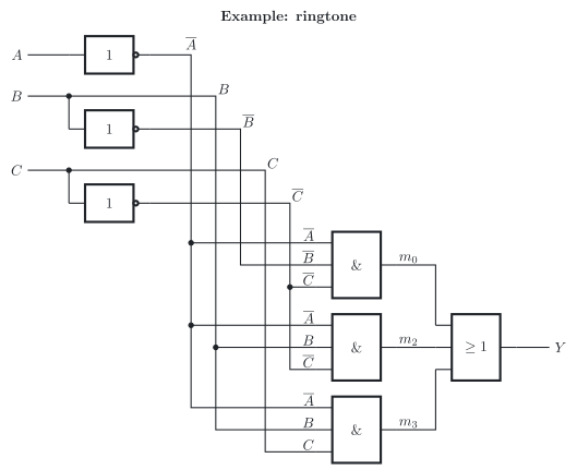
The circuit follows directly from the expression (figure): three inverters provide the negated inputs, three AND gates with three inputs each form the minterms, and an OR gate with three inputs combines them. At the inputs of each AND gate, you can read the literals of its minterm. Apart from the inverters, every signal passes through exactly two gates, first an AND and then an OR. Such a circuit is a two-level circuit (German: zweistufige Schaltung); its delay is that of two gates if the inputs are also available negated or if the delay of the inverters is neglected [12, p. 63]. The canonical DNF is always correct, but it uses the most gates possible for a truth table [5, p. 116].

2.3 Maxterms

The same truth table can also be read from its zeros. A maxterm (German: Volldisjunktion, Maxterm) is a sum, that is, an OR, that contains exactly one literal of each input variable and is 0 for exactly one combination of the inputs [5, p. 119]. Here, the rule for the literals is reversed: the variables that are 1 in this combination appear negated, the others as they are. Then all literals of the maxterm are 0 for this combination, and so is the OR. For every other combination, at least one variable has the other value; its literal is 1, and so is the OR. The maxterm $A+B+\overline{C}$, for example, is 0 only for $A=0$, $B=0$ and $C=1$. The maxterm of row $i$ is called $M_i$ [5, p. 119]. For three inputs, there are again eight. The column $Y$ shows the zeros of the ringtone, and section 2.4 needs exactly the maxterms of these rows:

Row $i$	$A$	$B$	$C$	$Y$	Maxterm $M_i$
0	0	0	0	1	$A+B+C$
1	0	0	1	0	$A+B+\overline{C}$
2	0	1	0	1	$A+\overline{B}+C$
3	0	1	1	1	$A+\overline{B}+\overline{C}$
4	1	0	0	0	$\overline{A}+B+C$
5	1	0	1	0	$\overline{A}+B+\overline{C}$
6	1	1	0	0	$\overline{A}+\overline{B}+C$
7	1	1	1	0	$\overline{A}+\overline{B}+\overline{C}$

Read the maxterm of row 1: ‘A or B or not C’. As a circuit, each maxterm is an OR gate with three inputs, with an inverter in front of every input that has to be 1.

2.4 The conjunctive normal form

Combined by AND, the maxterms of all rows with $Y=0$ deliver a 0 in exactly these rows and a 1 in all others. Conjunction is the mathematical name of the AND operation. In general, a conjunctive normal form (CNF, German: konjunktive Normalform, KNF) is any AND of OR terms, the sum terms (German: Summenterme). As with the DNF, canonical means that every term contains every variable: each term is then a complete maxterm. The AND of the maxterms of all rows with $Y=0$ is the canonical conjunctive normal form (German: kanonische konjunktive Normalform, KKNF) [5, p. 120], [12, p. 22]:

$$Y=M_{j_1}\cdot M_{j_2}\cdot \dots \cdot M_{j_l}$$

where:

• $Y$ is the output, 0 or 1
• $M_{j_1}$ to $M_{j_l}$ are the maxterms of the $l$ rows in which $Y=0$

For the ringtone, these are the rows with $Y=0$ in the table of section 2.3, rows 1, 4, 5, 6 and 7:

$$\begin{array}{rl}Y& =M_1\cdot M_4\cdot M_5\cdot M_6\cdot M_7\\ & =\left(A+B+\overline{C}\right)\cdot \left(\overline{A}+B+C\right)\\ & \cdot \left(\overline{A}+B+\overline{C}\right)\cdot \left(\overline{A}+\overline{B}+C\right)\\ & \cdot \left(\overline{A}+\overline{B}+\overline{C}\right)\end{array}$$

where:

• $Y$ is the output ‘ringtone audible’, 0 or 1
• $A$, $B$ and $C$ are the inputs ‘silent mode on’, ‘caller is a favourite’ and ‘Do Not Disturb on’, each 0 or 1

Each maxterm rules out one situation. $M_1$, for example, is 0 only when silent mode is off, Do Not Disturb is on and the caller is not a favourite; then it forces the output to 0.

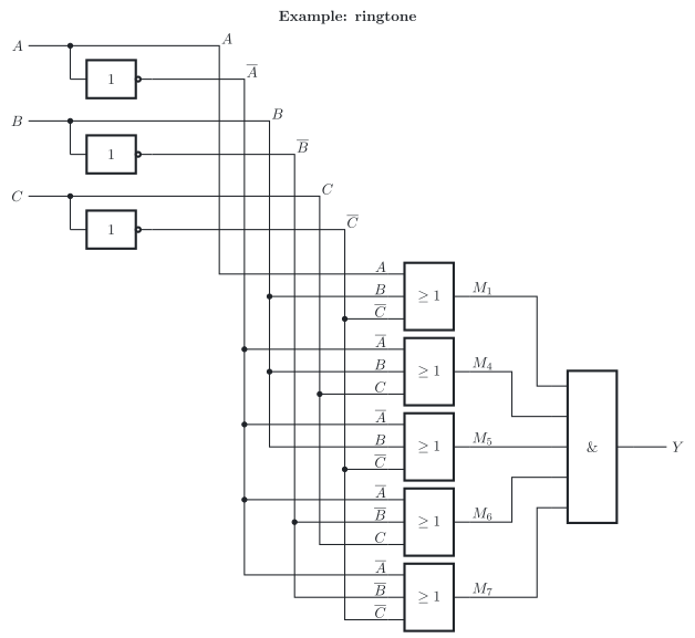
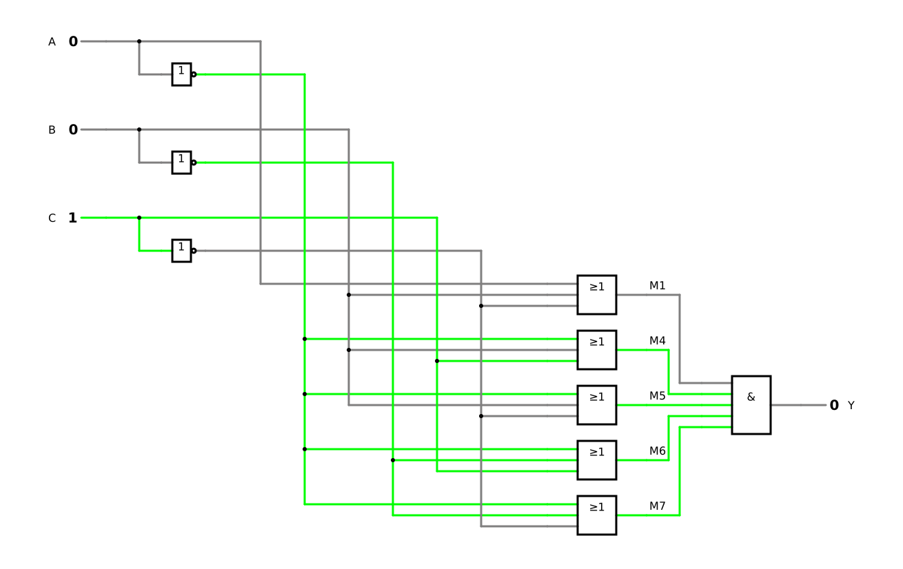
LaMeres calls the canonical CNF the canonical product of sums, or canonical product for short [5, pp. 119–120]. Its circuit is a two-level circuit as well, in the opposite order (figure): an OR gate for each maxterm and an AND gate that combines them. For the ringtone, it needs five OR gates with three inputs and an AND gate with five inputs. Both forms describe the same function: the DNF works by producing the ones, the CNF by producing the zeros [5, p. 120]. Since the ringtone has fewer ones than zeros, its canonical DNF is the shorter of the two.

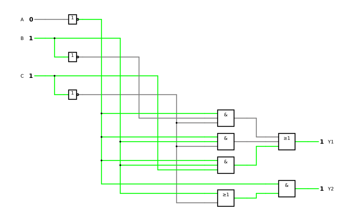
The simulation shows the same circuit, with the name of each maxterm at the output of its OR gate. It starts in row 1: silent mode off, caller not a favourite, Do Not Disturb on. Only $M_1$ is 0, and this single 0 makes the output of the AND gate 0: $Y=0$. Switch the inputs through all eight rows: in each row with $Y=0$, exactly one maxterm is 0, the one of this row; in the rows with $Y=1$, all five maxterms are 1.

Open in the simulator

Circuit as text (File → Import From Text…)

<cir f="1" ts="0.000005" ic="1.500424758475255" cb="50" pb="50" vr="5" mts="5e-11">
  <L x="96 80 48 80" f="2"/>
  <L x="96 208 48 208" f="2"/>
  <L x="96 336 48 336" f="2" p="1"/>
  <w x="96 80 144 80" f="0"/>
  <w x="144 80 320 80" f="0"/>
  <w x="144 80 144 128" f="0"/>
  <w x="144 128 176 128" f="0"/>
  <I x="176 128 240 128" f="0" sl="0.5" hi="5"/>
  <w x="240 128 384 128" f="0"/>
  <w x="96 208 144 208" f="0"/>
  <w x="144 208 448 208" f="0"/>
  <w x="144 208 144 256" f="0"/>
  <w x="144 256 176 256" f="0"/>
  <I x="176 256 240 256" f="0" sl="0.5" hi="5"/>
  <w x="240 256 512 256" f="0"/>
  <w x="96 336 144 336" f="0"/>
  <w x="144 336 576 336" f="0"/>
  <w x="144 336 144 384" f="0"/>
  <w x="144 384 176 384" f="0"/>
  <I x="176 384 240 384" f="0" sl="0.5" hi="5"/>
  <w x="240 384 640 384" f="0"/>
  <w x="320 80 320 432" f="0"/>
  <w x="320 432 736 432" f="0"/>
  <w x="384 128 384 512" f="0"/>
  <w x="384 512 384 592" f="0"/>
  <w x="384 592 384 672" f="0"/>
  <w x="384 672 384 752" f="0"/>
  <w x="384 512 736 512" f="0"/>
  <w x="384 592 736 592" f="0"/>
  <w x="384 672 736 672" f="0"/>
  <w x="384 752 736 752" f="0"/>
  <w x="448 208 448 448" f="0"/>
  <w x="448 448 448 528" f="0"/>
  <w x="448 528 448 608" f="0"/>
  <w x="448 448 736 448" f="0"/>
  <w x="448 528 736 528" f="0"/>
  <w x="448 608 736 608" f="0"/>
  <w x="512 256 512 688" f="0"/>
  <w x="512 688 512 768" f="0"/>
  <w x="512 688 736 688" f="0"/>
  <w x="512 768 736 768" f="0"/>
  <w x="576 336 576 544" f="0"/>
  <w x="576 544 576 704" f="0"/>
  <w x="576 544 736 544" f="0"/>
  <w x="576 704 736 704" f="0"/>
  <w x="640 384 640 464" f="0"/>
  <w x="640 464 640 624" f="0"/>
  <w x="640 624 640 784" f="0"/>
  <w x="640 464 736 464" f="0"/>
  <w x="640 624 736 624" f="0"/>
  <w x="640 784 736 784" f="0"/>
  <Or x="736 448 880 448" f="0" in="3"/>
  <Or x="736 528 880 528" f="0" in="3" o="5"/>
  <Or x="736 608 880 608" f="0" in="3" o="5"/>
  <Or x="736 688 880 688" f="0" in="3" o="5"/>
  <Or x="736 768 880 768" f="0" in="3" o="5"/>
  <w x="880 448 928 448" f="0"/>
  <w x="928 448 928 576" f="0"/>
  <w x="928 576 960 576" f="0"/>
  <w x="880 528 912 528" f="0"/>
  <w x="912 528 912 592" f="0"/>
  <w x="912 592 960 592" f="0"/>
  <w x="880 608 960 608" f="0"/>
  <w x="880 688 912 688" f="0"/>
  <w x="912 688 912 624" f="0"/>
  <w x="912 624 960 624" f="0"/>
  <w x="880 768 928 768" f="0"/>
  <w x="928 768 928 640" f="0"/>
  <w x="928 640 960 640" f="0"/>
  <And x="960 608 1104 608" f="0" in="5"/>
  <M x="1104 608 1152 608" f="2"/>
  <x x="12 86 22 89" f="0" si="16" te="A"/>
  <x x="12 214 22 217" f="0" si="16" te="B"/>
  <x x="12 342 23 345" f="0" si="16" te="C"/>
  <x x="884 440 906 443" f="0" si="16" te="M1"/>
  <x x="884 520 906 523" f="0" si="16" te="M4"/>
  <x x="884 600 906 603" f="0" si="16" te="M5"/>
  <x x="884 680 906 683" f="0" si="16" te="M6"/>
  <x x="884 760 906 763" f="0" si="16" te="M7"/>
  <x x="1172 614 1182 617" f="0" si="16" te="Y"/>
</cir>

2.5 Minterm and maxterm lists

Writing out canonical normal forms takes a lot of space. The minterm list (German: Mintermliste) only lists the numbers of the rows with $Y=1$, after a capital sigma, the sign for a sum [5, p. 118]. The maxterm list (German: Maxtermliste) lists the rows with $Y=0$ after a capital pi, the sign for a product [5, p. 122]. Both name the input variables in the order of the truth table, because this order determines the row numbers [5, pp. 118, 122]:

$$\begin{array}{rl}Y(A,B,C)& =\sum m(0,2,3)\\ Y(A,B,C)& =\prod M(1,4,5,6,7)\end{array}$$

where:

• $Y$ is the output ‘ringtone audible’, 0 or 1
• $A$, $B$ and $C$ are the inputs ‘silent mode on’, ‘caller is a favourite’ and ‘Do Not Disturb on’, each 0 or 1
• $m$ and $M$ stand for minterms and maxterms, followed by the numbers of their rows

Read: ‘Y of A, B and C is the sum of the minterms 0, 2 and 3’. The lists contain the same information as the truth table and the canonical normal forms, and you can switch between all of them without calculating [5, pp. 118, 122]. Every row number appears in exactly one of the two lists: a number that is missing in the minterm list is in the maxterm list, and vice versa [5, p. 123].

Two consequences matter in practice. First, the lists show at a glance which canonical normal form is shorter: with few ones, the DNF; with few zeros, the CNF. Second, the canonical normal forms are unique: for a given order of the variables, every function has exactly one minterm list. Two circuits with the same minterm list therefore do the same job, however different they look – section 5.2 uses this.

Besides the DNF and the CNF, there are further normal forms. The Reed–Muller form, for example, combines AND terms with XOR instead of OR. We only mention it; it plays no further role in this module.

3 Fewer gates, same function – Algebraic minimization

3.1 Why minimize?

With steps 1 to 3, the ringtone already has a circuit: the canonical disjunctive normal form (DNF) of section 2.2. It is always correct, but expensive: the canonical normal forms use the most gates that a truth table can need [5, pp. 116, 120]. Step 4 makes the circuit smaller without changing what it does (section 1.1). Minimization (German: Vereinfachung) turns an expression into an equivalent one with fewer operations. This reduces the number of gates, the area on the chip, the wiring and the power consumption of the circuit [5, p. 125].

Whether a circuit has become smaller can only be said with a measure of its effort. A simple measure is the number of gates and the number of their inputs. Inverters at the inputs are counted separately here, because in some circuits the input signals are also available negated [12, p. 63]. The canonical DNF of the ringtone needs three AND gates with three inputs each and an OR gate with three inputs: four gates with 12 gate inputs, plus three inverters for $\overline{A}$, $\overline{B}$ and $\overline{C}$ (figure in section 2.2). This is our starting point; section 5.1 compares the minimized circuit with it.

How do we get from the long expression to a short one? Two ways lead there. Sections 3.2 and 3.3 transform the expression with the theorems of Boolean algebra, which you know from DET-02, chapter 5. Chapter 4 of this lesson then shows a graphical way to the same result, the Karnaugh map [5, p. 126].

3.2 The uniting theorem

Algebraic minimization usually combines three theorems [5, p. 125]: the distributive property factors out a common part, the complements theorem replaces a sum such as $B+\overline{B}$ by 1, and the identity theorem removes the 1. Together, they form the uniting theorem of DET-02, 5.4: two products that differ in only one variable, which appears once as it is and once negated, unite into one product without this variable [5, p. 105].

In a canonical DNF, every term is a minterm and contains every variable. Two minterms that differ in only one variable can therefore always be united. In the ringtone, the minterms $m_0=\overline{A}\cdot \overline{B}\cdot \overline{C}$ and $m_2=\overline{A}\cdot B\cdot \overline{C}$ differ only in $B$, and the three theorems unite them, one after the other:

$$\begin{array}{rlrl}\overline{A}\cdot \overline{B}\cdot \overline{C}+\overline{A}\cdot B\cdot \overline{C}& =\overline{A}\cdot \overline{C}\cdot \left(\overline{B}+B\right)& & \text{commutative and distributive properties}\\ & =\overline{A}\cdot \overline{C}\cdot 1& & \text{commutative property, complements}\\ & =\overline{A}\cdot \overline{C}& & \text{identity}\end{array}$$

where:

• $A$, $B$ and $C$ are the inputs ‘silent mode on’, ‘caller is a favourite’ and ‘Do Not Disturb on’, each 0 or 1

Two terms with three literals each have become one term with two literals. Read: if silent mode and Do Not Disturb are both off, the phone rings, whether the caller is a favourite or not. The variable $B$ drops out because it has no influence in these two rows: in row 0 and in row 2 of the truth table, the phone rings either way. The Karnaugh map of chapter 4 builds on exactly this theorem: it arranges the minterms so that the pairs that can be united stand next to each other.

3.3 Minimizing with the theorems

The ringtone has three minterms, and the middle one, $m_2=\overline{A}\cdot B\cdot \overline{C}$, has a partner in each of the other two: it differs from $m_0$ only in $B$, as in section 3.2, and from $m_3=\overline{A}\cdot B\cdot C$ only in $C$. To unite it with both, we need it twice. Idempotence allows this, because a term ORed with itself stays the same, $m_2+m_2=m_2$, as in DET-02, 5.6:

$$\begin{array}{rlrl}Y& =\overline{A}\cdot \overline{B}\cdot \overline{C}+\overline{A}\cdot B\cdot \overline{C}+\overline{A}\cdot B\cdot C& & \\ & =\overline{A}\cdot \overline{B}\cdot \overline{C}+\overline{A}\cdot B\cdot \overline{C}+\overline{A}\cdot B\cdot \overline{C}+\overline{A}\cdot B\cdot C& & \text{idempotence}\\ & =\overline{A}\cdot \overline{C}\cdot \left(\overline{B}+B\right)+\overline{A}\cdot B\cdot \left(\overline{C}+C\right)& & \text{commutative and distributive properties}\\ & =\overline{A}\cdot \overline{C}\cdot 1+\overline{A}\cdot B\cdot 1& & \text{commutative property, complements}\\ & =\overline{A}\cdot \overline{C}+\overline{A}\cdot B& & \text{identity}\\ & =\overline{A}\cdot \left(B+\overline{C}\right)& & \text{distributive and commutative properties}\end{array}$$

where:

• $Y$ is the output ‘ringtone audible’, 0 or 1
• $A$, $B$ and $C$ are the inputs ‘silent mode on’, ‘caller is a favourite’ and ‘Do Not Disturb on’, each 0 or 1

The second line writes $m_2$ twice. The third line factors out the common part of each pair, the fourth replaces $\overline{B}+B$ and $\overline{C}+C$ by 1, and the fifth removes the ones: each pair has been united as in section 3.2, the first one loses $B$, the second one loses $C$. The fifth line is a minimized DNF with two product terms of two literals each. The screen in DET-02, 5.6 went the same way, from the canonical DNF $\overline{A}\cdot B+A\cdot \overline{B}+A\cdot B$ to the minimized DNF $A+B$. For the ringtone, the last line factors out $\overline{A}$ once more and saves a further gate: the minimized DNF of the fifth line needs two AND gates and an OR gate, the last line only an OR gate and an AND gate.

Read the last line: the phone rings if silent mode is off and if the caller is a favourite or Do Not Disturb is off. This is the description of section 1.2 in a single sentence. Section 5.1 turns this expression into a circuit.

Algebraic minimization has a drawback: you have to recognize where a theorem can be applied, and it is easy to overlook a possible minimization [5, p. 126]. Here, the trick of the second line is not obvious, and nothing tells you whether the result is minimal. For large expressions, computers therefore do the minimization [5, p. 126]; for us, the Karnaugh map makes the pairs visible at a glance.

4 Zeros and ones in a grid – The Karnaugh map

4.1 Neighbours in the grid

The Karnaugh map is the second, graphical way of step 4 (section 1.1). In DET-02, 2.6, you met the Karnaugh map as one of the seven forms of representation: the truth table arranged as a grid, with one cell for each combination of the inputs [5, p. 126]. Its cells are arranged so that neighbouring cells differ in exactly one input [5, pp. 126–127]. This is its whole secret: two neighbouring ones stand for two minterms that differ in only one variable, and by the uniting theorem, this variable drops out (section 3.2). The map shows such pairs at a glance, where algebra has to search for them.

Neighbours are cells that touch horizontally or vertically; cells that touch only diagonally are not neighbours [5, p. 127]. The edges count as well. In the map with three inputs, the first and the last column are neighbours, because their codes differ in only one input [5, p. 127] – as if the map were rolled into a cylinder.

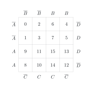
With four inputs, the map has four rows and four columns (figure). As in DET-02, 2.6, the labels show where each input is 1: $A$ on the left of the rows and $D$ on the right of them, $B$ above and $C$ below the columns. Now the top and the bottom row are neighbours as well, and so are the left and the right column [5, p. 128]. As a consequence, even the corners are neighbours: each corner is a neighbour of the corner in the same row and of the corner in the same column. In the figure, each cell shows the number of its minterm. The numbers do not run in order; row by row, the cells contain 0, 2, 6 and 4; 1, 3, 7 and 5; 9, 11, 15 and 13; 8, 10, 14 and 12. With the labels at the edges, however, you never need to remember this order: you read off where each input is 1.

Veitch and Karnaugh

In 1952, Veitch described a chart for minimizing logic functions. A year later, the physicist Karnaugh refined it at Bell Labs into the map that bears his name [5, p. 126]. In German, it is therefore called the Karnaugh-Veitch-Diagramm.

4.2 Loops of ones

To minimize with the map, you enter the outputs from the truth table and draw loops (German: Päckchen) around neighbouring ones. The rules are [5, pp. 130–132], [12, p. 54]:

1. A loop contains only ones and only neighbouring cells, also across the edges.
2. A loop contains 1, 2, 4, 8 or 16 cells, a power of two, and forms a rectangle, also across the edges.
3. Each loop is as large as possible.
4. Every one lies in at least one loop, and loops may overlap.

A loop whose ones all lie in other loops is not needed and is left out [5, pp. 137–138].

Each loop yields a product term. Go through the variables one by one: a variable that is 1 in all cells of the loop appears as it is, a variable that is 0 in all cells appears negated, and a variable that changes within the loop drops out [5, pp. 130–131]. A loop of two cells thus removes one variable, a loop of four removes two and a loop of eight removes three. The minimized expression is the OR of the product terms of all loops [5, p. 131]. Even the four corners of the map with four inputs (section 4.1) can form a loop of four [12, p. 55]: the cells of the minterms 0, 4, 8 and 12 all have $C=0$ and $D=0$, while $A$ and $B$ change, so such a loop yields $\overline{C}\cdot \overline{D}$.

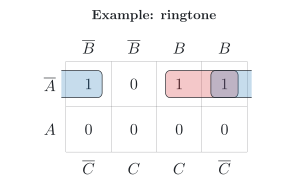
Our ringtone has its ones in the cells of the minterms 0, 2 and 3 (figure). The cells of 2 and 3 are neighbours in the upper row: $\overline{A}$ and $B$ are the same in both, while $C$ changes, so this loop yields $\overline{A}\cdot B$. The cells of 0 and 2 lie at the left and the right edge of the same row and are neighbours as well: $\overline{A}$ and $\overline{C}$ stay the same, while $B$ changes, so this loop yields $\overline{A}\cdot \overline{C}$. The cell of 2 lies in both loops, just as the minterm of row 2 was used twice in section 3.3:

$$Y=\overline{A}\cdot B+\overline{A}\cdot \overline{C}$$

where:

• $Y$ is the output ‘ringtone audible’, 0 or 1
• $A$, $B$ and $C$ are the inputs ‘silent mode on’, ‘caller is a favourite’ and ‘Do Not Disturb on’, each 0 or 1

The map yields the same minimized disjunctive normal form (DNF) as the algebra of section 3.3, without any trick: the overlap of the loops replaces the idempotence. LaMeres calls such a loop a prime implicant [5, p. 130]; prime implicants, and the question which loops a minimal expression really needs, follow in DET-04.

4.3 Loops of zeros

The map works just as well with its zeros [5, pp. 133–134]. Loops of neighbouring zeros follow the same rules and yield the sum terms of a minimized conjunctive normal form (CNF). The rule for the literals is reversed, as for the maxterms in section 2.3: a variable that is 1 in all cells of the loop appears negated, a variable that is 0 appears as it is, and a variable that changes drops out. The minimized expression is the AND of the sum terms of all loops [5, p. 134].

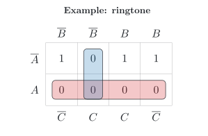
The ringtone has its zeros in the cells of the minterms 1, 4, 5, 6 and 7 (figure). The whole lower row forms a loop of four: there, $A=1$, while $B$ and $C$ change, so the sum term is $\overline{A}$. The remaining zero in the cell of 1 forms a loop of two with the cell of 5 below it: $B=0$ and $C=1$ in both, while $A$ changes, so the sum term is $B+\overline{C}$. Overlapping is allowed for zeros as well; the cell of 5 lies in both loops.

$$Y=\overline{A}\cdot \left(B+\overline{C}\right)$$

where:

• $Y$ is the output ‘ringtone audible’, 0 or 1
• $A$, $B$ and $C$ are the inputs ‘silent mode on’, ‘caller is a favourite’ and ‘Do Not Disturb on’, each 0 or 1

This is the expression in the last line of section 3.3, and the map has found it directly, with two loops. It is cheaper than the minimized disjunctive normal form (DNF) of section 4.2: an OR gate and an AND gate instead of two AND gates and an OR gate. Which form wins cannot be told in advance. It pays to draw both, the loops of ones and the loops of zeros, and to compare the effort as in section 3.1. The number of ones and zeros gives a first hint: the fewer cells a form has to cover and the larger its loops, the shorter it becomes.

4.4 Don’t cares

Sometimes the output of a function does not matter for some combinations of the inputs, for example because these combinations never occur [5, p. 139]. Such an output is called a don’t care (German: Don’t-Care-Term) and is marked with an X in the truth table and in the map [5, p. 139]. When you draw the loops, you may treat each X as a one or as a zero, whichever gives larger loops, or leave it out of the loops [5, p. 139].

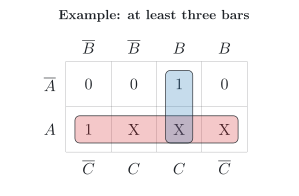
An example: suppose your smartphone shows the strength of the mobile signal as 0 to 4 bars and keeps this number as a binary number with the three bits $A$, $B$ and $C$, where $A$ has the highest weight. The codes 5, 6 and 7 then never occur. An app could, for example, upload large files over the mobile network only if the phone shows at least three bars. With $Y$ for ‘at least three bars’, the output is 1 for the codes 3 and 4; it is 0 for the codes 0 to 2; and it is a don’t care for the codes 5 to 7:

$$Y(A,B,C)=\sum m(3,4)+d(5,6,7)$$

where:

• $Y$ is the output ‘at least three bars’, 0 or 1
• $A$, $B$ and $C$ are the bits of the number of bars, $A$ with the highest weight, each 0 or 1
• $d$ stands for the don’t cares, followed by the numbers of their rows

Without the don’t cares, the two ones would not be neighbours, because the codes 011 and 100 differ in all three bits; the minimized expression would be the canonical $\overline{A}\cdot B\cdot C+A\cdot \overline{B}\cdot \overline{C}$. With the don’t cares treated as ones, the whole lower row becomes a loop of four, and the cell of 3 forms a loop of two with the cell of 7 below it (figure):

$$Y=A+B\cdot C$$

where:

• $Y$ is the output ‘at least three bars’, and $A$, $B$ and $C$ are the bits of the number of bars, each 0 or 1

An OR gate and an AND gate with two inputs each replace two AND gates with three inputs, an OR gate and three inverters.

Don’t cares need care, though: the finished circuit still delivers a definite value for these codes, here a 1 for the codes 5 to 7. If such a code occurs after all, because of a fault or a later change, the circuit reacts with this value. Use a don’t care only if the combination really never occurs or its output really does not matter. The heat pump offers the same situation: if the energy manager never sends the start command of Smart Grid Ready, the combination 1:1 never reaches the heat pump (DET-02, 6.6), and every circuit that evaluates the two signals may treat it as a don’t care.

4.5 The chequerboard: XOR

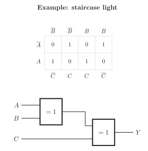
Not every function can be minimized with loops. Think of a staircase that connects three floors, with a light switch on each floor. The switches at the bottom and at the top are two-way switches, as in the two-way switching of DET-02, 4.3; the switch in the middle is an intermediate switch [16]. This intermediate switching (German: Kreuzschaltung) lets you switch the light from three places: whichever switch you flip, the light changes its state [16]. If we call the positions of the three switches $A$, $B$ and $C$, the light is on – with a suitable assignment of the positions – when an odd number of them is 1:

$A$	$B$	$C$	$Y$
0	0	0	0
0	0	1	1
0	1	0	1
0	1	1	0
1	0	0	1
1	0	1	0
1	1	0	0
1	1	1	1

The map of this function looks like a chequerboard [5, pp. 139–140] (figure): no two ones are neighbours, because flipping a single switch always changes the output. No loop can unite two cells, and the minimized disjunctive normal form (DNF) is the canonical one, with four minterms of three literals each.

The chequerboard pattern (German: Schachbrettmuster) reveals the XOR operation [5, pp. 139–140]. The XOR gate delivers a 1 if its two inputs differ; two XOR gates in a row deliver a 1 if an odd number of the three inputs is 1:

$$Y=A\oplus B\oplus C=\left(A\oplus B\right)\oplus C$$

where:

• $Y$ is the output ‘light on’, 0 or 1
• $A$, $B$ and $C$ are the positions of the three switches, each 0 or 1

Two XOR gates with two inputs each replace four AND gates with three inputs, an OR gate with four inputs and three inverters; in this module, an XOR gate always has two inputs. Written with XOR, the function is a simple case of the Reed–Muller form from section 2.5. The inverted chequerboard, with ones where an even number of inputs is 1, reveals the XNOR operation in the same way [5, pp. 140–141]. With three inputs, this is $Y=\overline{A\oplus B\oplus C}$, for example an XOR gate followed by an XNOR gate; two XNOR gates in a row would give the chequerboard again. Boolean algebra itself has no XOR operation [5, p. 139]; this is why the loops cannot find it, and why you have to look out for the pattern yourself.

5 Same job, different circuit? – Drawing and checking the circuit

5.1 Step 5: from the expression to the circuit

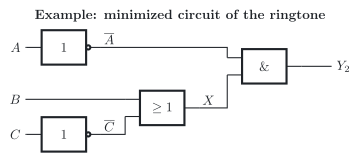
With the minimized expression, step 4 is complete. Step 5 turns the expression into a circuit, or describes it in VHDL (section 1.1). A minimized disjunctive normal form (DNF) or conjunctive normal form (CNF) becomes a two-level circuit directly, just like the canonical forms of chapter 2 [12, p. 63]. The last line of section 3.3 is such a form: the AND of the two sum terms $\overline{A}$ and $B+\overline{C}$, a minimized CNF. The Karnaugh map found the same expression with two loops of zeros (section 4.3). As in the canonical CNF of section 2.4, the first level consists of OR gates and the second of an AND gate. A sum term with a single literal needs no OR gate: $\overline{A}$ comes directly from an inverter.

The circuit (figure) therefore needs an inverter for $A$, an inverter for $C$, an OR gate for $B+\overline{C}$ and an AND gate that combines $\overline{A}$ with the output of the OR gate. To tell the two circuits of the ringtone apart, we call the output of this minimized circuit $Y_2$ and the output of the canonical DNF of section 2.2 $Y_1$. As in the analysis of DET-02, 6.1, we label the intermediate node at the output of the OR gate with $X$ [5, pp. 111–112]:

$$\begin{array}{rl}X& =B+\overline{C}\\ Y_2& =\overline{A}\cdot X=\overline{A}\cdot \left(B+\overline{C}\right)\end{array}$$

where:

• $X$ is the intermediate node at the output of the OR gate, 0 or 1
• $Y_2$ is the output of the minimized circuit, 0 or 1
• $A$, $B$ and $C$ are the inputs ‘silent mode on’, ‘caller is a favourite’ and ‘Do Not Disturb on’, each 0 or 1

Instead of drawing the circuit, you can describe it in VHDL, as in DET-02, 2.8; chapter 6 of this lesson does this for a complete design.

Step 5 also shows what minimizing has gained. Counted as in section 3.1:

Circuit	AND gates	OR gates	Gate inputs	Inverters
Canonical DNF $Y_1$	3	1	12	3
Minimized circuit $Y_2$	1	1	4	2

If the minimized circuit does the same job – section 5.2 checks this – it needs half the gates and a third of the gate inputs. In a single smartphone, this saving is tiny. A chip, however, contains a great many such functions, and the savings add up in area, power and cost.

5.2 Two circuits, one function?

Minimizing has replaced the circuit of the canonical DNF by a different, much smaller one. Before we use it, step 6 checks it (section 1.1): a single wrong line in the algebra or a wrongly drawn loop in the map would change the function, and nobody would see it in the circuit. We now have two circuits for the ringtone, and they look completely different:

$$\begin{array}{rl}{Y}_1& =\overline{A}\cdot \overline{B}\cdot \overline{C}+\overline{A}\cdot B\cdot \overline{C}+\overline{A}\cdot B\cdot C\\ Y_2& =\overline{A}\cdot \left(B+\overline{C}\right)\end{array}$$

where:

• $Y_1$ is the output of the canonical DNF of section 2.2, 0 or 1
• $Y_2$ is the output of the minimized circuit of section 5.1, 0 or 1
• $A$, $B$ and $C$ are the inputs ‘silent mode on’, ‘caller is a favourite’ and ‘Do Not Disturb on’, each 0 or 1

This is our second guiding question: two circuits look completely different – how can you prove that they do exactly the same job? There are three ways.

The first way compares the truth tables. It is the proof by exhaustion of DET-02, 5.3: each variable can only be 0 or 1, so you try every combination [5, p. 95], and no case is left out. Analyse the minimized circuit as in DET-02, 6.2: for each combination of the inputs, evaluate first the intermediate node $X$ and then the output $Y_2$ [5, p. 112]. For $Y_1$, you need not evaluate the long expression: the canonical DNF was read from the truth table of the ringtone, so its output column is the column $Y$ of section 1.2 of this lesson. Then compare the two outputs row by row:

$A$	$B$	$C$	$X=B+\overline{C}$	$Y_2=\overline{A}\cdot X$	$Y_1$
0	0	0	1	🟢1	🟢1
0	0	1	0	🟢0	🟢0
0	1	0	1	🟢1	🟢1
0	1	1	1	🟢1	🟢1
1	0	0	1	🟢0	🟢0
1	0	1	0	🟢0	🟢0
1	1	0	1	🟢0	🟢0
1	1	1	1	🟢0	🟢0

The two output columns agree in every row, so both circuits do the same job. A single differing row would prove the opposite (section 5.3).

The second way uses the minterm lists. $Y_2$ is 1 in rows 0, 2 and 3, so $Y_2=\sum m(0,2,3)$, the same list as for $Y_1$ (section 2.5). Since every function has exactly one minterm list, this proves it as well.

The third way transforms one expression into the other with Boolean algebra. Section 3.3 has already done this: each line there follows from the one before by a theorem, and a theorem never changes the function. The minimization itself is therefore a proof – provided that every line in it is correct.

The simulation shows both circuits, one above the other, driven by the same three inputs. Whatever you switch, the outputs $Y_1$ and $Y_2$ always show the same value.

Open in the simulator

Circuit as text (File → Import From Text…)

<cir f="1" ts="0.000005" ic="1.500424758475255" cb="50" pb="50" vr="5" mts="5e-11">
  <L x="96 96 48 96" f="2"/>
  <L x="96 160 48 160" f="2" p="1"/>
  <L x="96 288 48 288" f="2" p="1"/>
  <w x="96 96 160 96" f="0"/>
  <I x="160 96 224 96" f="0" sl="0.5" hi="5"/>
  <w x="224 96 288 96" f="0"/>
  <w x="96 160 128 160" f="0"/>
  <w x="128 160 352 160" f="0"/>
  <w x="128 160 128 224" f="0"/>
  <w x="128 224 160 224" f="0"/>
  <I x="160 224 224 224" f="0" sl="0.5" hi="5"/>
  <w x="224 224 416 224" f="0"/>
  <w x="96 288 128 288" f="0"/>
  <w x="128 288 480 288" f="0"/>
  <w x="128 288 128 352" f="0"/>
  <w x="128 352 160 352" f="0"/>
  <I x="160 352 224 352" f="0" sl="0.5" hi="5"/>
  <w x="224 352 544 352" f="0"/>
  <w x="288 96 288 416" f="0"/>
  <w x="288 416 288 496" f="0"/>
  <w x="288 496 288 576" f="0"/>
  <w x="288 576 288 656" f="0"/>
  <w x="352 160 352 512" f="0"/>
  <w x="352 512 352 592" f="0"/>
  <w x="352 592 352 688" f="0"/>
  <w x="416 224 416 432" f="0"/>
  <w x="480 288 480 608" f="0"/>
  <w x="544 352 544 448" f="0"/>
  <w x="544 448 544 528" f="0"/>
  <w x="544 528 544 720" f="0"/>
  <And x="640 432 784 432" f="0" in="3"/>
  <w x="288 416 640 416" f="0"/>
  <w x="416 432 640 432" f="0"/>
  <w x="544 448 640 448" f="0"/>
  <And x="640 512 784 512" f="0" in="3"/>
  <w x="288 496 640 496" f="0"/>
  <w x="352 512 640 512" f="0"/>
  <w x="544 528 640 528" f="0"/>
  <And x="640 592 784 592" f="0" in="3" o="5"/>
  <w x="288 576 640 576" f="0"/>
  <w x="352 592 640 592" f="0"/>
  <w x="480 608 640 608" f="0"/>
  <Or x="848 512 992 512" f="0" in="3" o="5"/>
  <w x="784 432 816 432" f="0"/>
  <w x="816 432 816 496" f="0"/>
  <w x="816 496 848 496" f="0"/>
  <w x="784 512 848 512" f="0"/>
  <w x="784 592 816 592" f="0"/>
  <w x="816 592 816 528" f="0"/>
  <w x="816 528 848 528" f="0"/>
  <M x="992 512 1040 512" f="2"/>
  <Or x="640 704 784 704" f="0" o="5"/>
  <w x="352 688 640 688" f="0"/>
  <w x="544 720 640 720" f="0"/>
  <And x="848 672 992 672" f="0" o="5"/>
  <w x="288 656 848 656" f="0"/>
  <w x="784 704 816 704" f="0"/>
  <w x="816 704 816 688" f="0"/>
  <w x="816 688 848 688" f="0"/>
  <M x="992 672 1040 672" f="2"/>
  <x x="12 102 22 105" f="0" si="16" te="A"/>
  <x x="12 166 22 169" f="0" si="16" te="B"/>
  <x x="12 294 23 297" f="0" si="16" te="C"/>
  <x x="1060 518 1079 521" f="0" si="16" te="Y1"/>
  <x x="1060 678 1079 681" f="0" si="16" te="Y2"/>
</cir>

5.3 Does the circuit do what it should?

In section 5.2, the minimized circuit passed the check against the canonical DNF, and thus against the truth table of the description, from which the canonical DNF was read. Without a second circuit, you compare a circuit directly with the description. A circuit fulfils the required function if its truth table agrees with the table of the description in every single row. A single row in which it deviates is enough to reject it: such a row is a counterexample (German: Gegenbeispiel).

Suppose a third design for the ringtone reads $Y_3=\overline{A}\cdot \overline{C}$: the phone rings if silent mode and Do Not Disturb are both off. The design looks plausible, and it is even smaller. Its minterm list, however, is shorter than the one that the description demands:

$$Y_3=\overline{A}\cdot \overline{C}=\sum m(0,2)\ne \sum m(0,2,3)$$

where:

• $Y_3$ is the output of the third design, 0 or 1
• $A$ and $C$ are the inputs ‘silent mode on’ and ‘Do Not Disturb on’, each 0 or 1

Row 3 is the counterexample: silent mode is off, Do Not Disturb is on and a favourite calls, so the description demands a 1, but the circuit delivers a 0. If someone from your family is among your favourites, their call at night stays silent. The designer has forgotten the exception: $Y_3$ consists of only one of the two product terms that section 3.3 found, and the term $\overline{A}\cdot B$, which lets the favourites through, is missing.

Four points help you to check a circuit systematically:

• Derive its truth table or its minterm list, as in DET-02, chapter 6.
• Compare it with the table of the description, row by row; one deviation is enough to reject the circuit.
• Look closely at the rows that describe exceptions, such as the favourites: the third design fails at such a row.
• If the description leaves a row open, clarify it before you judge the circuit (section 1.2).

In the simulator, you can switch the inputs through all combinations and compare the output with the table. With three inputs, these are eight combinations; with ten inputs, they would already be 1 024. For large circuits, tools therefore carry out the comparison automatically [5, pp. 161, 163] (section 6.3).

6 Sun for the hot water or for the battery? – A complete design

6.1 The rule and its truth table

Now we go through all six steps of section 1.1 with our heat pump and answer the last guiding question. In our example system, a photovoltaic (PV) system on the roof produces electricity, and a battery of lithium iron phosphate (LFP) cells stores surplus energy for later. The heat pump can store surplus energy as well, as heat in the hot-water tank. On a cold, sunny day like the one in the photo, the PV modules often deliver more power than the house needs at the moment. Where should the surplus go: into the battery or, through the heat pump, into the hot water?

Image by Qwen-Image 2.1

In our example system, an energy manager decides this. Through Smart Grid Ready, it can raise the set point of the hot water (DET-02, 6.6). Simplified, it follows a rule like this: the battery has priority until it is charged to 80 %. Then the surplus goes into the hot water, as long as the water is below its upper set point – unless the solar thermal collectors on the roof are heating it already. In all other cases, the surplus goes into the battery. We leave aside the heating of the house, the car and a small boiler in the kitchen, which in the real system also take surplus energy.

Step 1 defines the variables:

• $A$: there is a PV surplus; in the real system, more than 3.5 kW must have been fed into the power grid for ten minutes
• $B$: the battery is charged to at least 80 %
• $C$: the hot water is below its upper set point
• $D$: the solar thermal pump is running
• $Y$: the surplus goes into the hot water
• $Z$: the surplus goes into the battery

Step 2 sets up the truth table. Without a surplus, $A=0$, there is nothing to distribute, and both outputs are 0. With a surplus, exactly one of them is 1:

Row	$A$	$B$	$C$	$D$	$Y$	$Z$
0	0	0	0	0	0	0
1	0	0	0	1	0	0
2	0	0	1	0	0	0
3	0	0	1	1	0	0
4	0	1	0	0	0	0
5	0	1	0	1	0	0
6	0	1	1	0	0	0
7	0	1	1	1	0	0
8	1	0	0	0	0	1
9	1	0	0	1	0	1
10	1	0	1	0	0	1
11	1	0	1	1	0	1
12	1	1	0	0	0	1
13	1	1	0	1	0	1
14	1	1	1	0	1	0
15	1	1	1	1	0	1

In rows 8 to 11, the battery is below 80 % and has priority. In rows 12 and 13, the hot water has reached its upper set point; in row 15, the sun is heating it already. Only in row 14 does the surplus go into the hot water.

6.2 Minimizing both outputs

Steps 3 and 4 come together here: the Karnaugh map starts from the truth table and yields the minimized expressions directly [5, p. 126]. Output $Y$ has a single 1, in row 14. A single cell cannot be united with any other, so $Y$ remains a minterm:

$$Y=A\cdot B\cdot C\cdot \overline{D}$$

where:

• $Y$ is the output ‘surplus into the hot water’, 0 or 1
• $A$, $B$, $C$ and $D$ are the inputs ‘PV surplus’, ‘battery charged to at least 80 %’, ‘hot water below its upper set point’ and ‘solar thermal pump running’, each 0 or 1

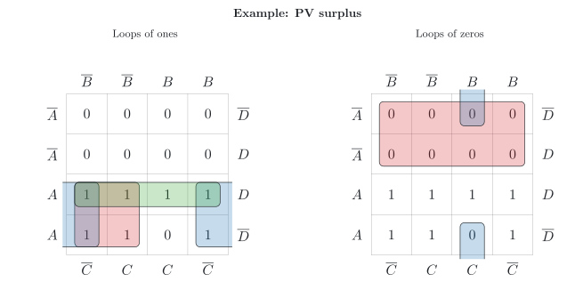
Output $Z$ has seven ones. Its canonical disjunctive normal form (DNF) would need seven AND gates with four inputs and an OR gate with seven inputs. In the map (figure, left), the ones form three loops of four:

• the four cells with $A=1$ and $B=0$, a square: $A\cdot \overline{B}$
• the four cells with $A=1$ and $C=0$, which lie in the left and the right column and are neighbours across the edge: $A\cdot \overline{C}$
• the four cells with $A=1$ and $D=1$, a whole row: $A\cdot D$

$$Z=A\cdot \overline{B}+A\cdot \overline{C}+A\cdot D$$

where:

• $Z$ is the output ‘surplus into the battery’, 0 or 1
• $A$, $B$, $C$ and $D$ are the inputs of section 6.1, each 0 or 1

The zeros give an even shorter result (figure, right). The eight zeros with $A=0$, the whole upper half of the map, form a loop of eight with the sum term $A$. The last zero, in the cell of 14, has a neighbour across the top and the bottom edge, the cell of 6; together, they yield the sum term $\overline{B}+\overline{C}+D$:

$$Z=A\cdot \left(\overline{B}+\overline{C}+D\right)$$

where:

• $Z$ is the output ‘surplus into the battery’, 0 or 1
• $A$, $B$, $C$ and $D$ are the inputs of section 6.1, each 0 or 1

An OR gate with three inputs and an AND gate with two inputs replace the eight gates of the canonical DNF.

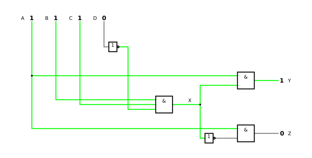
Both outputs can even share a gate. By De Morgan’s laws, $\overline{B}+\overline{C}+D$ is the negation of $B\cdot C\cdot \overline{D}$ (DET-02, 5.5). We introduce this product as an intermediate node $X$, which means ‘the hot water can take the surplus’:

$$\begin{array}{rl}X& =B\cdot C\cdot \overline{D}\\ Y& =A\cdot X\\ Z& =A\cdot \overline{X}\end{array}$$

where:

• $X$ is the intermediate node ‘the hot water can take the surplus’, 0 or 1
• $Y$ and $Z$ are the outputs ‘surplus into the hot water’ and ‘surplus into the battery’, each 0 or 1
• $A$, $B$, $C$ and $D$ are the inputs of section 6.1, each 0 or 1

Three AND gates and two inverters, one for $D$ and one for $X$, now do the work of the whole truth table. Minimizing several outputs together is a goal of its own in circuit design [12, p. 63]; shared terms like this save further gates.

6.3 VHDL, simulation and check

Step 5 describes the circuit for a programmable device in VHDL, as in DET-02, 6.4. The intermediate node $X$ becomes a signal of the architecture:

-- A: PV surplus, B: battery at 80 % or more
-- C: below upper set point
-- D: solar thermal pump on
-- Y: into the hot water, Z: into the battery
entity pv_surplus is
  port (A, B, C, D : in  bit;
        Y, Z       : out bit);
end entity;
 
architecture behaviour of pv_surplus is
  signal X : bit;  -- hot water takes the surplus
begin
  X <= B and C and not D;
  Y <= A and X;
  Z <= A and not X;
end architecture;

Each operator becomes a gate: the two and of the first assignment form the AND gate with three inputs, and each not becomes an inverter. The order of the three assignments does not matter, because they are concurrent.

Step 6 checks the circuit. In the simulation, you can switch the four inputs through all 16 combinations and compare both outputs with the truth table of section 6.1. Two conditions reveal errors quickly: without a surplus, both outputs must be 0, and with a surplus, exactly one of them must be 1.

Open in the simulator

Circuit as text (File → Import From Text…)

<cir f="1" ts="0.000005" ic="1.500424758475255" cb="50" pb="50" vr="5" mts="5e-11">
  <L x="96 64 96 16" f="2" p="1"/>
  <L x="176 64 176 16" f="2" p="1"/>
  <L x="256 64 256 16" f="2" p="1"/>
  <L x="336 64 336 16" f="2"/>
  <w x="336 64 336 112" f="0"/>
  <I x="336 112 400 112" f="0" sl="0.5" hi="5"/>
  <w x="400 112 416 112" f="0"/>
  <w x="416 112 416 320" f="0"/>
  <w x="176 64 176 288" f="0"/>
  <w x="256 64 256 304" f="0"/>
  <And x="464 304 608 304" f="0" in="3" o="5"/>
  <w x="176 288 464 288" f="0"/>
  <w x="256 304 464 304" f="0"/>
  <w x="416 320 464 320" f="0"/>
  <w x="608 304 656 304" f="0"/>
  <w x="656 304 656 240" f="0"/>
  <w x="656 240 736 240" f="0"/>
  <w x="656 304 656 416" f="0"/>
  <I x="656 416 720 416" f="0" sl="0.5" hi="5"/>
  <w x="720 416 736 416" f="0"/>
  <w x="96 64 96 208" f="0"/>
  <w x="96 208 96 384" f="0"/>
  <w x="96 208 736 208" f="0"/>
  <w x="96 384 736 384" f="0"/>
  <And x="736 224 880 224" f="0" o="5"/>
  <And x="736 400 880 400" f="0"/>
  <M x="880 224 928 224" f="2"/>
  <M x="880 400 928 400" f="2"/>
  <x x="60 22 70 25" f="0" si="16" te="A"/>
  <x x="140 22 150 25" f="0" si="16" te="B"/>
  <x x="220 22 231 25" f="0" si="16" te="C"/>
  <x x="300 22 311 25" f="0" si="16" te="D"/>
  <x x="616 296 626 299" f="0" si="16" te="X"/>
  <x x="948 230 958 233" f="0" si="16" te="Y"/>
  <x x="948 406 957 409" f="0" si="16" te="Z"/>
</cir>

With four inputs, the map still fits on a sheet of paper. A truth table with six inputs, however, already has 64 rows, and one with ten inputs has 1 024. For large expressions, tools therefore do the minimization [5, p. 126]: when they turn VHDL code into a circuit, they look for an inexpensive circuit themselves. Inside, they represent the functions in a way that suits a computer, for example as binary decision diagrams, and they check each intermediate result automatically [5, p. 163]. DET-04 shows the algorithm that a computer follows to minimize and what you do when a map becomes too large.

7 What have you learnt? – Summary and answers to the guiding questions

7.1 The building blocks of knowledge

• Representation of logic functions (normal forms): Every truth table can be written as a canonical disjunctive normal form (DNF), the OR of the minterms of its ones, or as a canonical conjunctive normal form (CNF), the AND of the maxterms of its zeros. Minterm and maxterm lists write them in short; for a given order of the variables, they are unique.
• Algebraic minimization: The distributive property, the complements theorem and the identity theorem, together with idempotence where a term is needed twice, turn a canonical normal form into a shorter expression with the same function.
• Minimization with the Karnaugh map: Neighbouring cells differ in exactly one input, also across the edges. Loops of 1, 2, 4 or 8 ones yield the product terms of a minimized DNF, loops of zeros the sum terms of a minimized CNF; don’t cares enlarge the loops, and a chequerboard reveals an XOR.

With these building blocks, you synthesize a circuit in six steps, from the description to the check against it, and you prove with the truth table or the minterm list whether a circuit fulfils the required function.

7.2 Answers to the guiding questions

How can a hand-drawn grid of zeros and ones make a logic circuit smaller and cheaper?
The Karnaugh map arranges the truth table so that neighbouring cells differ in exactly one input. Neighbouring ones can therefore be united: a loop of 2, 4 or 8 cells removes 1, 2 or 3 variables from its term. Fewer and shorter terms mean fewer gates and fewer gate inputs, and so a smaller and cheaper circuit.

Two circuits look completely different: how can you prove that they do exactly the same job?
Compare their truth tables row by row: if the outputs agree in every row, the circuits do the same job, and a single differing row proves the opposite. Equivalently, compare their minterm lists, which are unique for each function, or transform one expression into the other with Boolean algebra. For the ringtone, the canonical disjunctive normal form (DNF) with four gates and the circuit $\overline{A}\cdot \left(B+\overline{C}\right)$ with two gates have the same minterm list $\sum m(0,2,3)$.

On a cold, sunny day, when should the energy from the photovoltaic (PV) system go into the hot-water tank and when into the lithium iron phosphate (LFP) battery – and how do you turn that rule into a circuit that can be produced efficiently?
Into the hot-water tank only if there is a surplus, the battery is charged to at least 80 %, the water is below its upper set point and the solar thermal system is not heating it already: $Y=A\cdot B\cdot C\cdot \overline{D}$. In every other case with a surplus, the energy goes into the battery: $Z=A\cdot \left(\overline{B}+\overline{C}+D\right)$. The rule becomes a truth table, and the Karnaugh map minimizes it. Since both outputs share the term $B\cdot C\cdot \overline{D}$, three AND gates and two inverters do the whole job.

---

Where do I look things up? – Sources and references

All sources that I cite in this script with a number in square brackets, such as [5], are listed on the page References. There you will also find the books that I recommend for looking things up, the image licences and a note on the use of AI.

---

Exercises for this lesson

Exercise DET-03.01 – Normal forms
Exercise DET-03.02 – Algebraic minimization
Exercise DET-03.03 – Karnaugh maps
Exercise DET-03.04 – Repeated calls during Do Not Disturb
Exercise DET-03.05 – Heat pump boost with solar thermal collectors

---

Slides for this lesson

The slides of this lesson as PDF: Slides DET-03

---

⏭️ Continue with: DET-04 Minimization and hazards 🔗